Graphs
- Notes based on Graphs Series by William Fiset
- Pseudocode and lots of the images from above as well
Graph Introduction
Graph Terminology
- Undirected Graph: Graph where edges have no orientation. The edge (u, v) is the same as the edge (v, u).
- Directed Graph (Digraph): Edges have orientation. Edge from (u, v) is the edge from node u to node v.
- Weighted Graphs: Edges have weights to represent values like cost, distance, quantity, etc.
- Connected Component: The subgraph where it’s possible to get to any vertex from any vertex (but doesn’t have to be an edge between every vertex to every other vertex).
- The following graph has 3 connected components

- The following graph has 3 connected components
Tree
Connected undirected graph with no cycles. Equivalent definition: Connected graph with N nodes N-1 edges.
Examples:

Rooted Tree
- Tree that has a designated root node where every edge points either away from the root or towards the node.
- Out-Tree (Arborescence) : All edges point away from root
- In-Tree (Anti-Arborescence) : All edges point towards root (More common)

Directed Acyclic Graph (DAG)
Directed graph with no cycles
- Represent dependencies (class prereqs, scheduling, etc.)
- All out-trees are DAGs but not all DAGs are out-trees
- The difference between trees and DAGs is that nodes in DAGs can have multiple parents, while tree nodes can only have on parent.

Bipartite Graph
- Definition 1: Vertices can be split into two independent groups U, V such that every edge connects between U and V.
- Definition 2: Two colored graph
- Definition 3: No odd length cycles

Complete Graph
Unique edge between every pair of nodes.
- Complete graph with n vertices is denoted as the graph $K_n$
- Complete graphs are often seen as the worst case graph due to there being the maximum amount of edges

Graph Representation
Adjacency Matrix
| Pros | Cons |
|---|---|
| Space efficient for dense graphs | Requires $O(V^2)$ space |
| Edge weight lookup is $O(1)$ | Iterating over all edges takes $O(V^2)$ |
| Simplest graph representation |
Adjacency List
| Pros | Cons |
|---|---|
| Space efficient for sparse graphs | Less space efficient for denser graphs |
| Iterating over all edges is efficient | Edge weight lookup is $O(E)$ |
| Slight more complex graph representation |
Edge List
Unordered list of edges. Triplet (u, v, w) means “the cost from u to node v is w”.
| Pros | Cons |
|---|---|
| Space efficient for sparse graphs | Less space efficient for denser graphs |
| Iterating over all edges is efficient | Edge weight lookup is $O(E)$ |
| Very simple structure | Lacks structure, so seldom used |
Common Graph Theory Problems
Shortest Path
Shortest path from node A to node B
- BFS (only for unweighted), Dijkstra’s, Bellman-Ford, Floyd-Warshall, A*, etc.
Connectivity
Does there exist a path between node A to B
- Union find or DFS/BFS
Negative Cycles
Does a weighted digraph have negative cycles?
- Negative cycles are like a trap since the sum of the weighted edges keeps decreasing as you go through the cycle
- Bellman-Ford and Floyd-Warshall
Strongly Connected Components (SCC)
SCCs are self-contained cycles within a directed graph where each vertex in a given cycle can reach every other vertex in the same cycle.
- Tarjan’s Algorithm, Kosaraju’s Algorithm with DFS
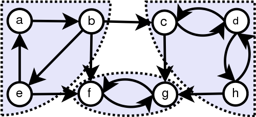
- a, b, e is a SCC and f, g is a SCC and c, d, h is a SCC
Traveling Salesman Problem
“Given a list of cities and the distance between pair of cities, what is the shortest possible route that visits each city exactly once and returns to the origin city?”
- NP Hard
- Held-Karp with Dynamic Programming, Branch and Bound, and approximation algorithms
Bridges
A Bridge/cut edge is any edge whose removal increases the number of connected components.
- Bridges can help identify weak points and bottlenecks
- The bolded edges are bridges since they would disconnect a part of the graph and create a new connected component

Articulation Points
Any node in a graph that increases number connected components when cut.
Minimum Spanning Tree (MST)
“Subset of edges of a connected, edge-weighted graph that connects all the vertices together, without any cycles and with the minimum possible total edge weight.”

- All MSTs have the same total cost, but MSTs on a graph are not always unique.
- Kruskal’s, Prims, etc.
Network Flow: Max Flow
With an infinite input source, how much “flow” can we push through the network?
- Edges can be roads with cars, pipes with water, or hallways with people. Flow would be the number of cars the roads can sustain in traffic, volume of water allowed in the pipes, and maximum number of people in hallways, respectively.
- Ford-Fulkerson, Edmonds-Karp, Dinic’s Algorithm
Depth First Search
- See https://jacobshin.com/notes/computer-science/data-structures/#depth-first-search
- Stuff Augmented DFS can do:
- Compute a graph’s Minimum spanning tree
- Check if graph is bipartite
- Find strongly connected components
- Topologically sort the nodes of a graph
- Find bridges and articulation points
- Find augmenting paths in a flow network?
- Generate mazes
Count Connected Components
Algorithm: Start a DFS at every node (unless it’s already visited) and mark all reachable nodes as being part of the same component. BFS also works in place of DFS.
Breadth First Search
Grids
- Grids are implicit graphs since you can determine a node’s neighbors (e.g. mazes, maps, etc.)
- Common approach is to convert grid to adjacency list/matrix
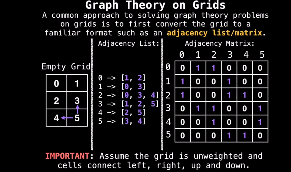
- Conversion isn’t strictly necessary in all cases; instead you can just use properties of the grid.
Shortest Path in Maze Grid
- For example, if you wanted to access adjacent vertices (neighboring cells in the grid):
# From https://youtu.be/KiCBXu4P-2Y
# Define the direction vectors for
# north, south, east, and west.
dr = [-1, +1, 0, 0]
dc = [0, 0, +1, -1]

for (i = 0; i < 4; i++):
  rr = r + dr[i]
  cc = c + dc[i]

  # Skip invalid cells. Assume R and
  # C for the number of rows and columns
  if rr < 0 or cc < 0: continue
  if rr >= R or cc >= C: continue

  # (rr, cc) is a neighboring cell of (r, c)
You can still use BFS to see if a grid based maze is solvable, just using the above to find adjacent vertices and puting the (x, y) pair of the neighbors in a queue. An alternative to putting an (x, y) pair into a single queue is to put x in one queue and y in a separate queue (works well for higher dimensional coordinates as well).
Topological Sort
- DAGs can model school class prereqs, program dependencies, event scheduling, etc.
- Topological orderings are not unique; there can be more than one topological orderings in a graph
- Graphs with cycles can’t have topological orderings since cyclic dependencies mean there’s no place to start
- To find if a graph is a DAG, you can use Tarjan’s Strongly Connected Component algorithm to find cycles
- Trees by definition don’t have cycles, so they have a topological ordering
- Pick off the leaves
- Keep removing the leaves of the new tree to get topological ordering
Algorithm
- Pick an unvisited node
- Beginning with the selected node, do a DFS exploring only unvisited nodes
- On the recursive callback of the DFS (when you backtrack/pop off the stack frame), add the current node to the topological ordering in reverse order
Shortest/Longest Path in DAGs
Shortest Path in DAGs
The Single Source Shortest Path (SSSP) problem can be solved on a DAG in $O(V + E)$. Dijkstra’s might not work for negative weights, but the following algo does and is faster.
-
Generates the shortest path from a source node for ALL other nodes
-
“Relax each edge”, keep updating the path if it’s better than what’s already there for each node (similar to dijkstra’s)
-
Go through each node in topological ordering and for each adjacent node update the table of paths if a better path is found
d = [infinity, infinity, ..., infinity] # Keeps track of shortest paths (distance from start node) for each node
d[start_node] = 0

Generate topological ordering

for node, n, in the topological ordering:
  for every node, v, adjacent to n:
    if d[n] + weight(n, v) < d[v]:
      d[v] = d[n] + weight(n, v)
Longest Path in DAG
- For a general graph finding the longest path is NP-Hard, but for a DAG it’s $O(V+E)$
- For DAG multiply edge values by -1 and find the shortest path and then multiply edge values by -1 again
Dijkstra’s Algorithm
- Dijkstra’s is a SSSP (Single Source Shortest Path)
- Specify a source node
- Get back the shortest path from the source to all other node
- Time Complexity can be $O(E\cdot \log(V))$
- Dijkstra constraint: All edges have to have non-negative edges weights
- Once a node has been visited, its optimal distance cannot be improved (greedy manner)
Lazy Algorithm
- Create “dist” array where distance is positive infinity. Mark distance to start node as 0.
- Maintain priority queue of key-value pairs of (node index, distance) which tell you which node to visit next based on which node has the min distance.
- Insert (s, 0) into priority queue and loop until PQ is empty, pulling out the next most promising pair (node index, distance), which is the one with the smallest distance.
- Iterate over all edges outwards from the current node and relax each edge appending to new key-value pair to the priority queue for every relaxation
visited = [false, false, ..., false]
dist = [infinty, infinity, ... infinity]
dist[start_node] = 0
PQ = []

PQ.add(start_node, 0)

while (PQ is not empty):
  v, oldDist = PQ.remove()
  visited[v] = true

  if dist[v] < oldDist: continue # This means this is a duplicate key-value pair. Means it's an old entry, so ignore it

  for every node, n, adjacent to node v:
    if visited[n] == true: continue

    if dist[v] + edge(v, n) < dist[n]:
      dist[n] = dist[v] + edge(n, v)

      PQ.add((n, dist[n]))

return dist
- Note how the distance is stored in two places, the dist array and in the value of the key-value Priority Queue. This is what makes the implementation lazy, since we have to delete outdated distances in the priority queue whenever we pull out a pair from the PQ and it is greater than what’s in the dist array.
- In this context, a visited node is the same thing as processed node
- Note how there can be multiple entries in the PQ with the same node and different distances. This is because updating a key-value entry in a PQ takes linear time (since the PQ is sorted by value, not by key), so the workaround is just to add a new entry and ignore the old one.
Finding the Shortest Path
-
The above doesn’t actually give you the shortest path, just the length of the paths
-
To actually get the path, add a
prev = [null, null, null ... null]array that keeps track of the node that comes before a node in the shortest path traversal -
Then set
prev[n] = vifdist[v] + edge(v, n < dist[n]and add areturn (dist, prev)at the end of the dijkstra function -
Then to find the shortest path, first make sure
dist[end_node] != infinity -
Then reconstruct the shortest path by starting at the
end_nodeand working backwards, using the prev array -
Return the path but reverse it since we worked backwards
Stopping Early
- If we’re only looking for the shortest path between two nodes, and we don’t need the shortest path from the source to ALL the other nodes, we can stop Dijkstra early once we visit the destination node, since once the destination node has been visited, its shortest distance will not change as more future nodes are visited.
- In the code, you can just add simple check to see if the node we processed is the end node
Eager Algorithm using Indexed Priority Queue
- Lazy version adds new key-value pairs $log(n)$ instead of updating values $O(n)$
- Lazy version is inefficient for dense graphs due to lots of stale key-value pairs
- In the Eager version, use a indexed priority queue to update the key-value pairs instead of just adding new ones
- Indexed priority queues allow updating a key-value pair (also called a decrease key operation) to be done much faster than linear time
D-ary Heap
- A D-ary heap can be used instead of an indexed-priority queue to make Dijkstra’s faster
- D-ary Heap is where each node has D children
- Faster update (decrease-key) operations
- Slower removals
- Faster updates and slower removals works well with Dijkstra’s since Dijkstra’s does more updates than removals
- D = E/V for optimal performance
- Leads to $O(E\cdot \log_{E/V}(V))$
The State of the Art Heap for Dijkstra’s
- Fibonacci Heap
- $O(E + V\log(V))$
- Impractical in practice since Fibonacci heaps are difficult to implement and has a large amortized constant overhead (so only useful for really large graphs)
Bellman-Ford (BF) Algorithm
- Another SSSP (Single Source Shortest Path) algo
- Finds shortest path from one node to any other node
- $O(EV)$
- Worse than Dijkstra’s $O((E+V)\log(V))$
- Use BF when Dijkstra’s fails with negative cycles (Dijkstra would be stuck in an infinite loop as it finds better and better paths)
- Application of negative cycles: Arbitrage in financial markets
Algorithm
- E = Number of edges
- V = Number of vertices
- S = starting node
- D = array of size V that tracks the best distance from S to each node
- Set every entry in D to $+\infty$
- Set D[S] = 0
- Relax each edge V-1 times
for (i = 0; i < V-1; i++):
  for edge in graph.edges:
    // Relax edge (update D with shorter path
    if (D[edge.from] + edge.cost < D[edge.to])
      D[edge.to] = D[edge.from] + edge.cost

// Find nodes caught in negative cycle
for (i = 0; i < V-1; i++):
  for edge in graph.edges:
    if (D[edge.from] + edge.cost < D[edge.to])
      D[edge.to] = -infinity
Floyd Warshall Algorithm
- All-Pairs Shortest Path (APSP): Shortest path between all pairs of nodes
- $O(V^3)$ only good for graphs with a few hundred nodes
- Detects negative cycles and works with negative edges
- Bad for regular shortest path tho
Graph Setup
- Best way is using a 2d Adjacency Matrix, where m[i][j] represents the weight of the edge from node i to node j.
- If there is no edge from i to j, then set edge m[i][j] = $+\infty$
- IMPORTANT: If the programming language doesn’t support a constant infinity such that $\infty + \infty = \infty$, then don’t use 2^32 - 1 as infinity since it will cause an integer overflow; using a large constant like 10^7 might be better.
- The goal of FW is to eventually consider going through all possible intermediate nodes on paths of different lengths
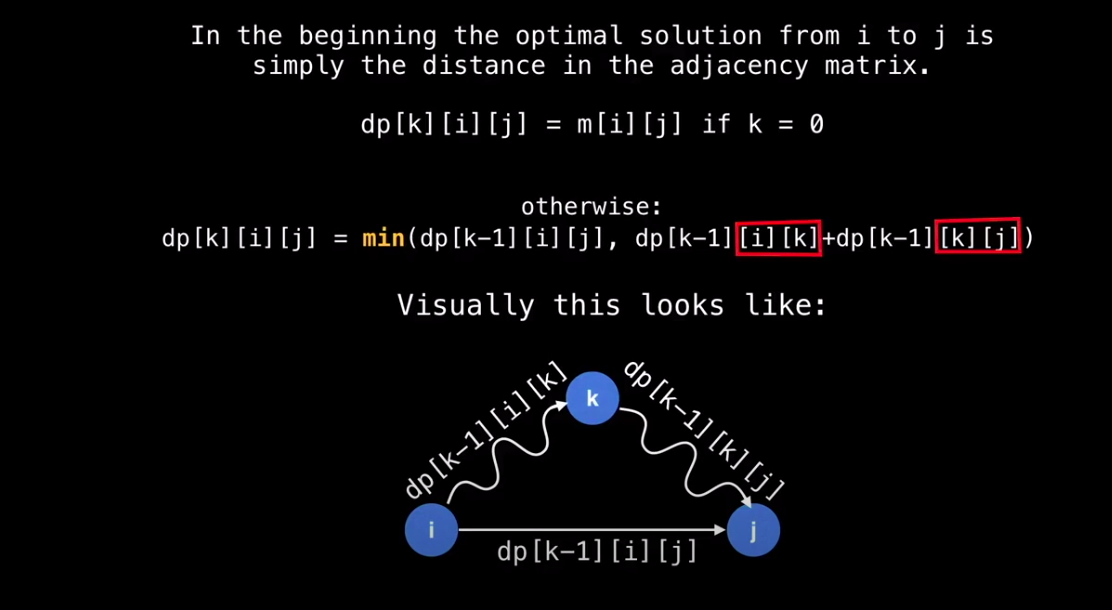
Memo Table
- Use Dynamic Programming (DP) using a memo table
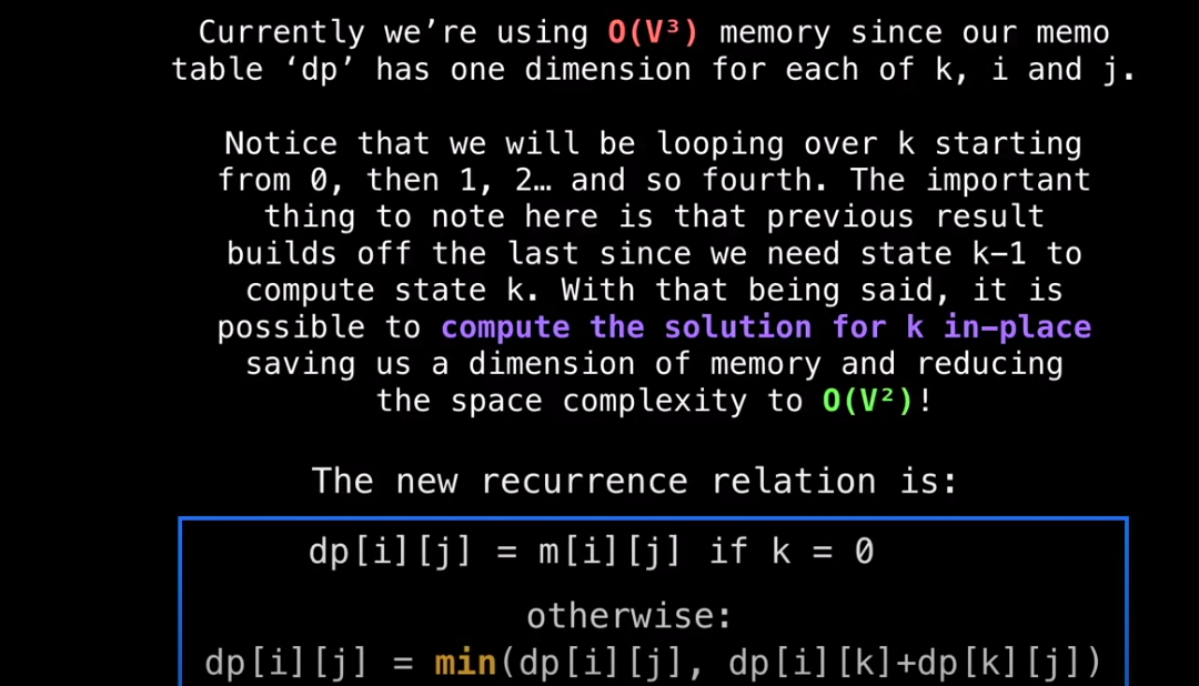
- In this case the memo table is a 3d matrix of size n x n x n
dp[k][i][j] = shortest path from i to j routing through nodes {0, 1, … k-1, k}
-
Start with k=0, then k=1, then k=2, …
-
This gradually builds up the optimal solution routing through 0, then all optimal solutions routing through 0 and 1, then all optimal solutions routing through 0, 1, 2, etc. up until n-1.
-
dp[n-1] is the 2d Matrix solution we’re after
n = size of adjacency matrix
dp = memo table with the APSP solution
next = matrix used to reconstruct shortest path

function floydWarshall(m):
  # Setup copies over values from m into dp
  # and sets next[i][j] = j if m[i][j] != +infinity
  setup(m)

  for (k:= 0; k < n; k++):
    for (i:=0; i < n; i++):
      for (j:=0; j < n; j++):
        if (dp[i][k] + dp[i][k] < dp[k][j]):
          dp[i][j] = dp[i][k] + dp[k][j]
          next[i][j] = next[i][k]

  # Detect and propogate negative cycles
  propogateNegativeCycles(dp, n)

  # Return APSP matrix
  return dp
- If a shortest path goes through a negative cycle, it is compromised and thus is invalid. To find these negative cycles, run FW a second time but if the distance can be improved set the optimal distance to be -infinity
- Every edge (i, j) marked with -infinity is either part of or reaches into a negative cycle.
function propogateNegativeCycles(dp, n):
  for (k:= 0; k < n; k++):
    for (i:=0; i < n; i++):
      for (j:=0; j < n; j++):
        if (dp[i][k] + dp[i][k] < dp[k][j]):
          dp[i][j] = -infinity
          next[i][j] = -1
- To reconstruct a shortest path
function reconstructPath(start, end):
  path = []

  if dp[start][end] == +infinity: return path
  at = start

  for (; at != end; at = next[at][end]):
    # If at is -1, then the shortest path is stuck in a negative cycle
    if at == -1: return null

    path.add(at)

  if next[at][end] == -1: return null

  path.add(end)
  return path
Bridges and Articulation Points
- Bridge: Edge that increases number of connected components if removed
- Articulation Point: Node that increases the number of connected components when removed
Bridge Algorithm
-
Low-Link value is the smallest id reachable from a node using forward and backward edges
-
Do a depth first search and label each node with an unique id that you keep incrementing as you go to more nodes
-
Find the low link value for each node
-
If id(e.from) < lowlink(e.to), then you have a bridge
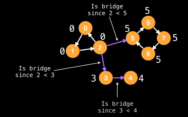
- This algorithm works since the definition of a bridge really just describes when you don’t have another edge going back to the node where the bridge starts. If you have another edge looping back to that node, you would have a low link value at least equal to the starting node’s id.
- The above algo does one DFS and V more DFSs to find all the low link values, so you have $O(V(V+E))$.
- However, a single pass of DFS can update the low-link values, giving $O(V+E)$
id = 0
g = adjacency list
n = size of the graph

ids = [0, 0, ..., 0]                         # length n
low = [0, 0, ..., 0]                         # length n
visited = [false, false, false, ..., false]  # length n

function findBridges():
  bridges = []

  for (i = 0; i < n; i++):
    if (!visited[i]):
      dfs(i, -1, bridges)
  return bridges

function dfs(at, parent, bridges):
  visited[at] = true
  id++
  low[at] = ids[at] = id

  # For each edge from node 'at' to node 'to'
  for (to: g[at]):
    if to == parent: continue
      if (!visited[to]):
        dfs(to, at, bridges)
        low[at] = min(low[at], low[to])
        if (ids[at] < low[to]):
          bridges.add((at, to))

      else:
        # If we've already visited the 'to' node, there's still a chance
        # that the low link value might have to be changed to the id of 'to'
        low[at] = min(low[at], ids[to])
Articulation Point Algorithm
- On a connected component with three or more vertices, if an edge (u, v) is a bridge, then either either u or v is an articulation point.
- The above condition doesn’t capture all articulation points since it’s possible for articulation points to exist without bridges nearby)
- For the callback
low[at] = min(low[at], low[to])after the DFS, ifid(e.from) == lowlink(e.to), then there is a cycle - The presence of a cycle also implies an articulation point
- The only exception when
id(e.from) == lowlink(e.to)fails is when the starting node has 0 or 1 outgoing directed edges.
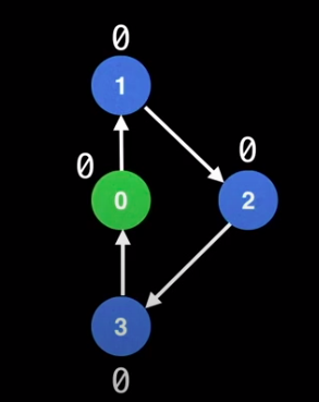
- Here, the starting node (green) has only 1 outgoing edge, so the condition fails and there’s no articulation point
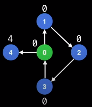
- However, when there’s more than one outgoing edge, the node can escape the cycle and become an articulation point
- For the callback
# Global variables accessible from any function
id = 0
g = adjacency list
n = size of the graph
outEdgeCount = 0

ids = [0, 0, ..., 0]                         # length n
low = [0, 0, ..., 0]                         # length n
visited = [false, false, false, ..., false]  # length n
isArt = [false, false, ..., false]           # length n

function findArtPoints():
  for (i = 0; i < n; i++):
    if (!visited[i]):
      outEdgeCount = 0 # Reset
      dfs(i, i, -1)
      isArt[i] = (outEdgeCont > 1)
  return isArt

function dfs(root, at, parent):
  if (parent == root): outEdgeCount++;

  visited[at] = true
  id++
  low[at] = ids[at] = id

  # For each edge from node 'at' to node 'to'
  for (to: g[at]):
    if to == parent: continue
      if (!visited[to]):
        dfs(to, at, bridges)
        low[at] = min(low[at], low[to])

        if (ids[at] == low[to]):
          isArt[at] = true
        if (ids[at] < low[to]):
          isArt[at] = true

      else:
        # If we've already visited the 'to' node, there's still a chance
        # that the low link value might have to be changed to the id of 'to'
        low[at] = min(low[at], ids[to])
Strongly Connected Components (SCC)
- Self-Contained cycles within a directed graph where every vertex in the given cycle can eventually reach every other vertex in the same cycle
- All nodes in a the same SCC have the same low link values, but only if DFS traversal is done in the right order
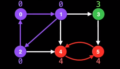
Tarjan’s Algorithm
- Tarjan’s algorithm maintains a set (most times a stack) of valid nodes from which to update low-link values from
- Nodes are added to teh stack of valid nodes as they’re explored for the first time
- Nodes are removed from the stack each a complete SCC is found
- If u and v are nodes we’re exploring
- To update u’s low link value to node v’s low link value, there has to be a graph of edges from u to v and node v must be on the stack
- Still $O(V+E)$
Algorithm
- Mark the id of each node as unvisited
- Start DFS anywhere. Assign id and low-link value. Mark as visited and add to seen stack
- On DFS callback, if the node we were going to is on the stack, then set low link of the node we’re at to min of at node’s low link and to node’s low-link
if (onStack[to]): low[at] = min(low[at], low[to]
- After visiting all neighbors in the current DFS call, if the current node started a connected component, then pop nodes off stack until current node is reached. (We know a node started a connected component if its id equals its low link value)
UNVISITED = -1
n = number of nodes in graph
g = adjacency list with directed edges

id = 0        # Used to give each node an id
sccCount = 0  # Used to count number of SCCs found

# Index i in these arrays represents node i
ids = [0, 0, ...0, 0]
low = [0, 0, ...0, 0] # Keeps track of low-links for all the n nodes

onStack = [false, false, ..., false]
stack = an empty stack data structure

function findSccs():
  for (i = 0; i < n; i++):
    ids[i] = UNVISITED

  for (i = 0; i < n; i++):
    if (ids[i] == UNVISITED):
      dfs(i)

  return low

function dfs(at):
  stack.push(at)
  onstack[at] = true
  ids[at] = low[at] = id++

  # Visit all neighbors & min low-link on the callback
  for (to: g[at]):
    if (ids[to] == UNVISITED):
      dfs(to)
    if (onStack[to]):
      low[at] = min(low[at], low[to])

  # After visiting all the neighbors of "at"
  # if we're at the start of a SCC, empty the seen stack
  # until we're back to the start of the SCC
  if (ids[at] == low[at]):
    for (node = stack.pop(); ; node = stack.pop()):
      onStack[node] = false
      low[node] = ids[at]
      if (node == at): break
    sccCount++
Traveling Salesman Problem (TSP)
- Reworded Problem: Given a complete graph with weighted edges (as adjacency matrix), what is the Hamiltonian cycle (path that visits every node only once) of minimum cost?
- NP-Complete: No known algorithm that runs in polynomial time
Brute Force Solutin
- Compute the cost of every possible tour. Try all possible permutations of node orderings which takes $O(n!)$
Dynamic Programming
- Reduces $O(n!)$ to $O(n^2 2^n)$
- Makes graphs up to 23 nodes feasible to solve the TSP for most home computers
Steps
- Pick a node $0 \le S < N$ to be the starting node, S, for the tour
- Compute the optimal solution when we have a path where n = 2, in other words a partial path with one edge. For this we need two things
- The set of visited nodes in the subpath
- The index of the last visited node in the path
- The above form the dynamic programming state. Since there are N possible nodes that could have visited last and 2^N possible subsets of visited nodes, the space needed to store the answer is $O(N2^N)$ since we need to store every possible combination for DP
- Note that we store the set of visited nodes in a single 32-bit integer to save space instead of an array
- To solve paths of length $3 \le n \le N$, we’re going to take the solved subpaths from n-1 which are cached, and add another edge extending to a node which hasn’t been visited from the last visited node
# m - 2D adjacency matrix of the graph
# S - The start node (0 <= S < N)

function tsp(m, S):
  N = matrix.size()

  # Initialize memo table
  # Fil table with null values or +infinity
  memo = 2D table of size N by 2^N

  setup(m, memo, S, N)
  solve(m, memo, S, N)

  minCost = findMinCost(m, memo, S, N)
  tour = findOptimalTour(m, memo, S, N)

  return (minCost, tour)

# Only generates tours with path length n=2 (two nodes)
function setup(m, memo, S, N):
  for (i = 0; i < N; i++):
    if i == S: continue

    # Store the optimal value from node S
    # to each node i (this is given as input
    # in the adjacency matrix m).
    memo[i][1 << S | 1 << i] = m[S][i]

    # Bits at "index" of S and "index" of i to 1 and the rest are zero
    # If S was 5 and i was 4, then the 5th and 4th bit are set so 10000 | 1000 = 11000
    # The memo[i] subarray keeps track of the visited nodes in a tour
    # and the i keeps track of the node visited last that we're keep incrementing

function solve(m, memo, S, N):
  # r keeps track of the number of nodes in a partial tour (gets incremented until N)
  for (r = 3; r <= N; r++):
    # The combinations function generates all bit sets
    # of size N with r bits set to 1. For example,
    # combinations(3, 4) = {011, 1011, 1101, 1110}
    for subset in combinations(r, N):
      # If S is not in the subset, then disgard that subset since it is invalid
      # since the subset doesn't contain our starting node
      if notIn(S, subset): continue

      # next is the next node we're going to
      for (next = 0; next < N; next++):
        # Check if the subset we generated has the next node in it
        # Basically run this loop body for every ndoe in the subset
        if next == S || notIn(next, subset): continue

        # The sbuset state without the next node
        state = subset ^ (1 << next)

        minDist = +infinity

        # 'e' is short for end node
        # Generate all possible end nodes and see which one is best
        for (e = 0; e < N; e++):
          # Invalid end node
          if (e == S || e == next || notIn(e, subset)):
            continue

          newDistance = memo[e][state] + m[e][next]
          if (newDistance < minDist):
            minDist = newDistance

        memo[next][subset] = minDist


function notIn(i, subset):
  # Check if the ith bit is 0
  return ((1 << i) & subset) == 0

function findMinCost(m, memo, S, N):
  # END_STATE is a bitmask with all N bits set to 1
  END_STATE = (1 << N) - 1

  minTourCost = +infinity

  for (e = 0; e < N; e++):
    if (e == S): continue

    tourCost = memo[e][END_STATE] + m[e][S]

    if tourCost < minTourCost: minTourCost = tourCost

  return minTourCost

function findOptimalTour(m, memo, S, N):
  lastIndex = S
  state = (1 << N) - 1 # end state
  tour = array of size N+1

  # Work backwards
  # Start with end state and remove the nodes one by one to get path
  for (i = N-1; i >=1; i--):
    index = -1
    # Find next node in path (in reverse order)
    for (j = 0; j < N; j++):
      if j == S || notIn(j, state): continue
      if (index == -1) index == j
      prevDist = memo[index][state] + m[index][lastIndex]
      newDist = memo[j][state] + m[j][lastIndex]
      if (newDist < prevDist) index = j

    tour[i] = index
    state = state ^ (1 << index) # remove the index node from the state since we're going backwards
    lastIndex = index

  tour[0] = tour[N] = S # Tour ends and starts at S
  return tour
Eulerian Paths
- Eulerian Path: Path of edges that visits all the edges in a graph exactly once.
- Eulerian Circuit: Eulerian path where the start and end are the same node
- If you know that an eulerian circuit exists, you can start on any node
| Eulerian Circuit | Eulerian Path | |
|---|---|---|
| Undirected Graph | Every vertex has an even degree. | Either every vertex has even degree or exactly two vertices have odd degree (start and end nodes) |
| Directed Graph | Every vertex has equal indegree and outdegree. | At most one vertex has outdegree-indegree = 1 and at most one vertex has indegree - outdegree = 1 and all other vertices have equal in and out degrees. |
- Requirement for paths/circuits is that all vertices with nonzero degree need to belong to a single connected component
Finding Eulerian Paths (Hierholzer’s Algorithm)
-
Determine if an eulerian path exists using the table
-
For directed graphs, we have to start at the node with exactly one extra outgoing edge and the end has to be the node with exactly one extra incoming edge
-
If we just do a regular DFS, even when starting at the right node and we know an Eulerian path exists, it doesn’t give us an Eulerian path
- Modify the DFS so that when you get “stuck” (no more out degrees to go to that aren’t yet visited), backtrack and add the nodes to a stack.
-
$O(E)$ since computing in/out degrees + DFS are both linear in number of edges
# Global/class scope variables
n = number of vertices in graph
m = number of edges in graph
g = adjacency list of the directed graph

in = [0, 0, ..., 0]  # length n
out = [0, 0, ..., 0] # length n

path = empty integer linkd list data structure

function fundEulerianPath():

  countInOutDegrees()
  if not graphHasEulerianPath(): return null

  dfs(findStartNode())

  if path.size() == m+1: return path
  return null

function countInOutDegrees():
  for edges in g:
    for edge in edges:
      out[edge.from]++
      in[edge.to]++

function graphHasEulerianPath():
  start_nodes, end_nodes = 0, 0

  for (i = 0; i < n; i++):
    if (out[i] - in[i]) > 1 or (in[i] - out[i])> 1):
      return false
    else if out[i] - in[i] == 1:
      start_nodes++
    else if in[i] - out[i] == 1:
      end_nodes++
    return (end_nodes == 0 and start_node==0) or (end_nodes == 1 and start_node == 1)

function findStartNode():
  start = 0
  for (i = 0; i < n; i++):
    # Unique starting node
    if out[i] - in[i] == 1: return i

    # Start at any node with an outgoing edge (so we don't start on a singleton node)
    if out[i] > 0: start = i


# The out array serves two purposes
# 1. track whether there are outgoing edges
# 2. Index into the adjacency list to select next outgoing edge
function dfs(at):
  # While the current node stil has outgoing edges
  while (out[at] != 0):

    # Select the next unvisited outgoing edge
    next_edge = g[at].get(--out[at])
    dfs(next_edge.to)

  path.insertFirst(at)
Minimum Spanning Tree (MST)
- Minimum Spanning Tree: The subset of the edges in the graph which connects all vertices (without cycles) while minimizing total edge cost for an undirected graph with weighted edges
- MSTs aren’t necessarily unique for a graph, meaning there can be multiple valid solutions with the same edge cost
- A MST can only exist if all the nodes are part of a single connected component
- For an undirected graph we can store it as a directed graph with one incoming edge and outbound edge per edge in the undirected graph
Prim’s MST Algorithm
-
Greedy, works well for dense graphs
-
Doesn’t parallelize well
-
Lazy Version: $O(E \cdot \log(E))$
-
Eager version: $O(E\cdot \log(V))$
Lazy Prim’s MST Algo
Steps
- Maintain a min Priority Queue (PQ) that sorts edges by min edge cost. Used to determine next node to visit and the edge to get to that node.
- Start the algo at s. Mark s as visited and iterate over all edges of s and add them to PQ.
- While the PQ is not empty and a MST has not been formed, dequeue the next edge from the PQ.
- If dequeued edge is outdated (i.e. node it points to has already been visited), then skip and poll again
- Otherwise mark the current node as visited and add the edge to the MST
- Iterate over the current node’s edges and add all its edges to PQ. Do not add edges to PQ that have already been visited.
- We know that the algorithm is done when the number of edges in the MST is one less than the number of nodes (definition of a tree)
Eager Prim’s MST Algo
- Instead of “blindly inserting edges into a PQ which could later become stale”, the eager version tracks (node, edge) key-value pairs that can easily be updated and polled
- Each node in the graph is paired with only one of its incoming edges for a MST (except start node)
- Instead of adding edges to the PQ as we iterate over the edges, in the eager version, we relax (update) the destination node’s most promising incoming edge using an Indexed Priority Queue (IPQ)
- IPQ = PQ + Hashmap and supports polling and updating in logarithmic time
- Since there are V (node, edge) pairs for this algo in the IPQ, the poll/update operations will be $O(\log(V))$
- Thus the total time complexity would be $O(E\cdot \log(V))$ since we need to poll/update for every edge
Steps
- Create a min IPQ of size V that sorts vertex-edge pairs (v, e) based on the min edge cost of e. By default all vertices v have a best value of (v, null) in the IPQ
- Start algorithm on the start node ‘s’ (any node). Mark s as visited and relax all edges of s. Relax means update the entry for node v in the IPQ from $(v, e_{old})$ to $(v, e_{new})$ if the new edge $e_{new}$ from u to v has a lower cost than $e_old$.
- While the IPQ is not empty and MST has not been formed, dequeue the next best (v, e) pair.
- Mark node v as visited and add edge e to the MST
- Relax all edges of v while making sure not to relax any edge pointing a node which has already been visited
n = # Number of nodes in the graph
ipq = # IPQ data structure, stores (node index, edge object) pairrs
      # Edge objects consist of {start node, end node, edge cost} tuples
      # IPQ sorts (node index, edge object) pairs based on min edge cost
g = # graph adjacency list

visited = [false, ..., false] # visited[i] tracks whether node i has been visited or not, size n

function eagerPrims(s = 0):
  m = n - 1 # number of total edges that should be in MST

  # edgeCount is current number of edge in the partial MST
  edgeCount, mstCost = 0, 0
  mstEdges = [null, ..., null] # size m

  relaxEdgesAtNode(s)

  while (!ipq.isEmpty() and edgeCount != m):
    destNodeIndex, edge = ipq.dequeue

    mstEdges[edgeCount++] = edge
    mstCost += edge.cost

    relaxEdgesAtNode(destNodeIndex)

  if edgeCount != m:
    return (null, null)
  return (mstCost, mstEdges)

function relaxEdgesAtNode(currentNodeIndex):
  visited[currentNodeIndex] = true

  edges = g[currentNodeIndex]

  for (edge: edges):
    destNodeIndex = edge.to

    if visited[destNodeIndex]: continue

    if !ipq.contains(destNodeIndex):
      ipq.insert(destNodeIndex, edge)
    else:
      # Try improving cheapest edge entry in IPQ if already in there
      ipq.decreaseKey(destNodeIndex, edge)
Kruskal’s Algorithm
- Select an edge of G of minimum weight
- Select a remaining edge of G of minimum weight
- Select any remaining edge of G of minimum weight that does not form a cycle with the previously selected edges
- Repeat 3. until n-1 edges have been selected (MST formed)
Max Flow Ford Fulkerson
- Question: With an infinite input soure, how much “flow” can we push through the network without exceeding the capacity of any edge?
- Two special nodes: source and sink
- Solution to question finds the flow for each edge to maximize flow for the total graph/network. Initially, the flow is 0 for each edge.
- Remaining Capacity:
e.capacity - e.flow - Augmenting Path: Path of edges in the residual graph with remaining capacity greater than zero from the source s to the sink t.
- Bottleneck: Smallest edge on the path (find this by subtracting current flow from capacity)
- Augmenting the Flow: Updating the flow values of the edges along augmenting path
- For forward edges, this means increasing the flow by the bottleneck value
- For back edges (called residual edges in this case), decrease the flow along each edge by the bottleneck value. A residual edge is in the opposite direction for every edge of the augmenting path
- Residual edges exist so that we can “undo” bad augmenting path decisions that don’t lead to maximum flow
- Every edge in the graph also starts out with a residual edge with flow/capacity of 0/0
- Residual Graph: The graph which also contains residual edges along with the regular edges
- The algorithm continues finding augmenting paths and augments the flow until no more augmenting paths from s to t exist.
- The sum of the bottlenecks fond in each augmenting path is equal to the max flow.
- Time complexity is dependent on how we find the augmenting paths
- If augmenting paths are found with DFS then the time complexity is $O(fE)$, where $f$ is maximum flow and $E$ is number of edges
Other Implementations of Ford-Fulkerson
- Edmonds-Karp: Use BFS to find augmenting paths, $O(E^2 V)$
- Capacity Scaling: Heuristic to pick larger paths first, $O(E^2 \log(U))$
- Dinic’s Algorithm: Uses combination of DFS + BFS to find augmenting paths, $O(V^2 E)$
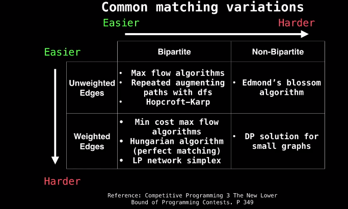
Unweighted Bipartite Graph Matching - Network Flow
- Bipartite Graph: Vertices can be split into two independent groups U, V such that every edge connects between U and V.
- Other definitions: The graph is two colorable or there is no cycle with an odd length
- Maximum Cardinality Bipartite Matching (MCBM): When we’ve maximized the pairs that can be matched with each other. What we’re usually interested in
Planar Graphs
- Planar Graph: Graph that can be drawn on one plane without any edges crossing/intersecting.
Euler’s Formula for Connected Planar Graphs
$$ v - e + r = 2$$
where v is the number of vertices, e is the number of edges, and r is the number of regions.
Proof
- Case 1: Graph is tree so use the fact that v=n and e=n-1
- Case 2: Removing edges until there is only one region turns the graph into a tree so that there are only $e-(r-1)$ edges
Other Properties
- $3r \le 2e$
- $e \le 3v - 6$
Image Credits
- David Eppstein
- Maksim
- Dcoetzee
- Rest of the graph diagrams based on Mr. Fiset’s videos