Class Description

Textbook: Differential Equation and Linear Algebra by Stephen W. Goode and Scott A. Annin

2.1: Matrix Definitions and Properties

• m x n matrix
• 3 x 4 matrix in the example below
  $$
  A = \begin{bmatrix}
  a_{11} & a_{12} & a_{13} & a_{14} \\
  a_{21} & a_{22} & a_{23} & a_{24} \\
  a_{31} & a_{32} & a_{33} & a_{34} \\
  \end{bmatrix}
  $$

$$ A = [a_{ij}]$$

Equality

Matrices $A$ and $B$ are equal if the following are true:

1. Same dimensions
2. $a_{ij} = b_{ij} \ \ \ \ \forall i, j \ \ \ 1 \le i \le m, \ \ 1 \le j \le n$

Vectors

• Row Vector: A $1 \cross n$ matrix
  $$
  \overrightarrow{a}= \vb{a} = A = \begin{bmatrix}
  a_1 & a_2 & a_3 & a_4 \\
  \end{bmatrix}
  $$

• Column Vector: A $n \cross 1$ matrix
  $$
  \overrightarrow{a} = \vb{a} = A = \begin{bmatrix}
  a_1 \\
  a_2 \\
  a_3 \\
  a_4 \\
  \end{bmatrix}
  $$

• The elements of a row or column vector are called the components

• Denoted via an arrow or in bold: $\vb{v}$ or $\overrightarrow{v}$

• A list of row vectors arranged in a row will always consist of column vectors, and a list of vectors arranged in a column will consist of row vectors

  • Example
    $$ \vb{a_1} = \begin{bmatrix} -1 \\ -7 \end{bmatrix}, \vb{a_2} = \begin{bmatrix} 0 \\ -5 \end{bmatrix}, \vb{a_3} = \begin{bmatrix} -2 \\ 4 \end{bmatrix}$$

$$ \begin{bmatrix} \vb{a_1} & \vb{a_2} & \vb{a_3} \end{bmatrix} = \begin{bmatrix} -1 & 0 & -2\\ -7 & -5 & 4\end{bmatrix}$$

Transposition

• Interchange row vectors and column vectors
  $$ a_{ij}^T = a_{ji}$$
• Example

$$ A = \begin{bmatrix} -1 & 0 & -2\\ -7 & -5 & 4\end{bmatrix}$$
$$ A^T = \begin{bmatrix} -1 & 7 \\ 0 & -5 \\ -2 & 4\end{bmatrix}$$

Square Matrices

• Square Matrix: An $n\cross n $ matrix
• Main Diagonal: $a_ii \ \ , 1\le i \le n $
• Trace: $tr(A) = a_{11} + a_{22} + … + a_{nn}$
• Lower Triangular: $a_{ij} = 0$ when $i < j$
  $$ A = \begin{bmatrix} -5 & 0 & 0\\ 0 & 4 & 0 \\ 2 & -2 & -7 \end{bmatrix}$$
• Upper Triangular: $a_{ij} = 0$ when $i > j$
  $$ A = \begin{bmatrix} 3 & 3 & 4\\ 0 & -5 & 1 \\ 0 & 0 & 9\end{bmatrix}$$
• Diagonal Matrix: $d_{ij} = 0$ whenever $i \neq j$
  $$ D = \begin{bmatrix} 0 & 0 & 0\\ 0 & -2 & 0 \\ 0 & 0 & 9\end{bmatrix}$$
• Symmetric: $A^T = A$
  $$ D = \begin{bmatrix} 0 & 2 & 3\\ 2 & 0 & 4 \\ 3 & 4 & 1\end{bmatrix}$$
• Skew-Symmetric: $A^T = -A$
  $$ D = \begin{bmatrix} 0 & 2 & 3\\ -2 & 0 & 4 \\ -3 & -4 & 1\end{bmatrix}$$

2.2: Matrix Algebra

Matrix Addition

• $A+B = [a_{ij} + b_{ij}]$

Properties

1. $A + B = B + A$ (Commutative)
2. $A + (B + C) = (A + B) + C$ (Associative)

Scalar Multiplication

• Scalar: Real or complex number
• Scalar Multiplication: If $s$ is a scalar, then $sA = [sa_{ij}]$

Properties

• (if $s$ and $t$ are scalars while $A$ and $B$ are matrices)

1. $1A = A$
2. $s(A+B) = sA + sB$
3. $(s + t)A = sA + tA$
4. $s(tA) = (st)A = (ts)A = t(sA)$

Subtraction

$$ A-B = A+(-1)B $$

Zero Matrix

• Matrix full of all zeros $0_{m\cross n}$
• Denoted with just a $0$ if dimensions are clear

Properties

1. $A + 0 = A$
2. $A - A= 0$
3. $0A = 0$

Multiplication

• If $A = [a_{ij}]$ is an $m \cross n$ matrix, $B = [b_{ij}]$ is an $n \cross p$ matrix, and $C = AB$, then
  $$ c_{ij} = \sum_{k=1}^{n} a_{ik}b_{kj} \ \ \ \ \ \ 1 \le i \le m, \ \ \ 1 \le j \le p$$

Properties

1. $A(BC) = (AB)C$
2. $A(B + C) = AB + AC$
3. $(A + B)C = AC + BC$
4. $AB \neq BA$

• Proof
  $$ (A+B)C_{ij} = \sum_{k=1}^{n} (a_{ik} + b_{ik}) c_{kj} = \sum_{k=1}^{n} a_{ik} c_{kj} + \sum_{k=1}^{n} b_{ik} c_{kj} $$
  $$ = (AC)_{ij} + (BC)_{ij} $$
  $$ = (AC + BC)_{ij}$$

Thus $(A+B)C = AC +BC$

Identity Matrix

• $I_n$: Main diagonals are just 1’s and zeros everywhere else
• Example
  $$ I_3 = \begin{bmatrix} 1 & 0 & 0\\ 0 & 1 & 0 \\ 0 & 0 & 1\end{bmatrix}$$

Kronecker Delta

• A function that gives the values for the identity matrix
  $$
  \delta_{ij} =
  \begin{cases}
  1 & i = j \\
  0 & i \neq j
  \end{cases}
  $$

Properties of Identity Matrix

1. $A_{m\cross n} I_n = A_{m \cross n}$
2. $I_m A_{m \cross p} = A_{m \cross p}$

• Proof: Use $\delta_{ij}$ in proof and definition of multiplication

Properties of Transpose

1. $(A^T)^T = A$
2. $(A + C)^T = A^T + C^T$
3. $(AB)^T = B^T A^T$

• Proof
  $$ (AB)^T_{ij} = (AB)_{ji}$$
  $$ = \sum_{k=1}^n a_{jk} b_{ki}$$
  $$ = \sum_{k=1}^{n} b_{ki} a_{jk} = \sum_{k=1}^{n} b_{ik}^T a^T_{kj}$$
  $$ = (B^T A^T)_{ij}$$

Properties of Triangular Matrices

• The product of two lower triangular matrices is a lower triangular matrix (and the same applies to upper triangular matrices)

The Algebra and Calculus of Matrix Functions

• Matrices can have functions as their elements instead of just scalars
• If $A$ and $B$ are matrices:

1. $\frac{dA}{dt} = \left[\frac{da_{ij}(t)}{dt}\right]$
2. $\frac{d}{dt}(AB) = A\frac{dB}{dt} + \frac{dA}{dt}B$
3. $\int_a^b A(t) dt = \left[\int_a^b a_{ij}(t) dt\right]$

2.3: Systems of Linear Equations

System of Linear Equations

$$ a_{11}x_1 + a_{12} x_2 + … + a_{1n}x_n = b_1$$
$$ a_{21}x_1 + a_{22} x_2 + … + a_{2n}x_n = b_2$$
$$ \vdots$$
$$ a_{m1}x_1 + a_{m2} x_2 + … + a_{mn}x_n = b_m$$

• System Coefficients: $a_{ij}$

• System Constants: $b_j$

  • Scalars
  • Correspond to $x_1, x_2, …, x_n$ (unknowns)

• Homogeneous: If $b_i = 0 \forall i$

• Solution: Ordered $n$-tuple with values for the unknowns ($x_1, x_2, x_3, …, x_n$)

• Solution Set: Set of all solutions to the system

• If there are two equations with two unknowns, we have two lines, so there can only be the following solutions:

  1. No solution
  2. One solution (one intersection point)
  3. Infinitely many solutions (the lines overlap or are the same)

• Similarly, with three equations and three unknowns, we have three planes, so there can only be the following solutions

  1. No solution
  2. One solution (Three planes intersect at one point)
  3. Infinitely Many Solutions (the three planes intersect at one line)
  4. Infinitely Many Solutions (the three planes are the same)

• All systems can only have one of the three above solution possibilities (no solution, one solution, or infinitely many solutions)

• Consistent: At least one solution to system

• Inconsistent: No solution to a system

• Matrix of Coefficients
  $$ A = \begin{bmatrix} a_{11} & a_{12} & … & a_{1n} \\ a_{21} & a_{22} & … & a_{2n} \\ \vdots \\ a_{m1} & a_{m2} & … & a_{mn}\end{bmatrix}$$

• Augmented Matrix:
  $$ A = \begin{bmatrix} a_{11} & a_{12} & … & a_{1n} & b_1 \\ a_{21} & a_{22} & … & a_{2n} & b_2 \\ \vdots \\ a_{m1} & a_{m2} & … & a_{mn} & b_m\end{bmatrix}$$

Vector Formulation

If we have the following:
$$ a_{11}x_1 + a_{12} x_2 + … + a_{1n}x_n = b_1$$
$$ a_{21}x_1 + a_{22} x_2 + … + a_{2n}x_n = b_2$$
$$ \vdots$$
$$ a_{m1}x_1 + a_{m2} x_2 + … + a_{mn}x_n = b_m$$

The vector formulation:
$$ \begin{bmatrix} a_{11} & a_{12} & … & a_{1n} \\ a_{21} & a_{22} & … & a_{2n} \\ \vdots \\ a_{m1} & a_{m2} & … & a_{mn}\end{bmatrix} \begin{bmatrix} x_1 \\ x_2 \\ \vdots \\ x_n \end{bmatrix} = \begin{bmatrix}b_1 \\ b_2 \\ \vdots \\ b_m \end{bmatrix}$$
$$ \vb{x} = \begin{bmatrix} x_1 \\ x_2 \\ \vdots \\ x_n \end{bmatrix}, \ \ \ \ \vb{b} = \begin{bmatrix}b_1 \\ b_2 \\ \vdots \\ b_m \end{bmatrix}$$
$$ A\vb{x} = \vb{b}$$

• Right-Hand Side Vector: $\vb{b}$
• Vector of Unknowns: $\vb{x}$

Notation

• The set of all ordered $n$-tuples of real numbers $(c_1, c_2, c_3, c_4, …, c_n)$ is denoted with $\mathbb{R}^n$
• For scalar values that are reals:
  $$ (x_1, x_2, …, x_n) \Longleftrightarrow \begin{bmatrix}x_1 & x_2 & … & x_n\end{bmatrix} \Longleftrightarrow \begin{bmatrix}x_1 \\ x_2 \\ \vdots \\ x_n \end{bmatrix}$$
• Tuples, row vectors, and column vectors are basically interchangeable in this context

Differential Equations

$$ \frac{d\vb{x}}{dt} = A(t) \vb{x}(t) + \vb{b}(t)$$

2.4: Row-Echelon Matrices and Elementary Row Operations

• Method for solving a system by reducing a system of equations to a new system with the same solution set, but easier to solve

Row-Echelon Matrix (REF)

Let A be a $m \cross n$ matrix with the following conditions

1. All zero rows of A (if any) are grouped at the bottom
2. The leftmost non-zero entry of every non-zero row is 1 (called the leading 1 or pivotal 1)
3. The leading 1 of a non-zero row below the first row is to the right of the leading 1 in the row above it

$$
\begin{bmatrix}
0 & 1 & … \\
0 & 0 & 0 & 1 & … \\
0 & 0 & 0 & 0 & 1 & … \\
0 & 0 & 0 & 0 & 0 & 0 & 0 & 0 & 1 & … \\
0 & 0 & 0 & 0 & 0 & … & 0 & 0 & 0 \\
0 & 0 & 0 & 0 & 0 & … & 0 & 0 & 0
\end{bmatrix}
$$

• Values after the leading 1 can be any value
• Pivotal Columns are columns where there is a leading 1

Elementary Row Operations

1. Permute row $i$ and $j$
2. Multiply row $i$ by a non-zero scalar $k$
3. Add the multiple $kR_j$ of row $j$ to $R_i, \ \ \ \ i \neq j, \ \ k \in \mathbb{R}$

• $A \sim B$ denotes that $B$ was obtained using one of the above operations
• The elementary row operations are reversible

Reduced Row Echelon Form (RREF)

• Same as REF but with only 0’s above every leading 1

Rank

• Rank(A) = number of pivotal columns = number of leading 1’s = number of non zero rows in REF form
• Every row equivalent REF has the same rank
• Every RREF of a matrix is the same, but not all row equivalent REF of a matrix are the same

2.5: Gaussian Elimination

• Gaussian Elimination: To solve a system, use elementary row operations to convert a matrix to REF. Convert matrix back into corresponding equations and solve.

• Gauss-Jordan Elimination: Convert to RREF and solve.

• Always either no solution, infinite solutions, or one solution

• If there is a leading 1 in the last row, there are no solutions since the system is inconsistent

• Homogeneous: $\overrightarrow{b} = 0$ Always has one solution or more.

• Free variables: Correspond to a non-pivotal column, means there are infinite solutions to system

• Non-Free variable: Correspond to a pivotal column

Theorem 2.5.9

Let $A$ is a coefficient $m \cross n$ matrix. $A^\#$ is the augmented matrix

1. If $rank(A) < rank(A^\#)$, then the system is inconsistent
2. If $rank(A) = rank(A^\#)$, then the system is consistent

• $rank(A) = n$ if and only if there is only one solution
• $rank(A) < n $ if and only if there is an infinite amount of solutions (free variables exist)

Corollary 2.5.11

For a homogeneous system, if $m < n$, then there is an infinite amount of solutions.

Proof

We know $rank(A) = rank(A^\#)$ since it’s a homogeneous system.
We also know $rank(A) \le m$ for any system. If $m < n$, then $rank(A) < n$ by transitivity.
By Theorem 2.5.9, the system has an infinite amount of solutions

Remark

The inverse is not true. There can still be an infinite amount of solutions if $m \ge n$ for a homogeneous system

2.6: The Inverse of a Square Matrix

When $A$ and $B$ are both $n \cross n$ matrices:
$$ AB = I_n \land BA = I_n$$
this chapter is about finding what $B$ is and if $B$ even exists.

Potential application of $B$: Solving a system $A\overrightarrow x= \overrightarrow b$
$$ A\overrightarrow x= \overrightarrow b$$
$$ (BA)\overrightarrow x= \overrightarrow Bb$$
$$ \overrightarrow x = B\overrightarrow b$$

We can solve for $\overrightarrow{x}$ simply by multiplying $B$ and $\overrightarrow{b}$. However, in practice this is slow, so it isn’t really used much.

Theorem 2.6.1

Theorem: There is only one matrix $B$ for a corresponding $A$.

Proof:
$$ AB = BA = I_n$$
$$ AC = CA = I_n$$
$$ C = CI_n = C(AB) $$
$$ C = (CA)B = I_n B = B $$
$$ C = B $$
(Uniqueness proof). See these notes

$$ AA^{-1} = A^{-1}A = I_n $$
If $A^{-1}$ exists, then it’s called the inverse and $A$ is called invertible

• Nonsingular Matrix: Sometimes called invertible
• Singular Matrix: Sometimes called non-invertible or degenerate

Remark: $A^{-1}$ does not mean $\frac{1}{A}$

Theorem 2.6.5

Theorem: If $A^{-1}$ exists, then the $n \cross n$ system of linear equations $A \overrightarrow{x} = \overrightarrow{b}$ has a unique solution $\vb{x} = A^{-1} \vb{b} \ \ \forall b \in \mathbb{R}^n$

Proof: Verify that $\vb{x} = A^{-1} \vb{b}$ is a solution with direct substitution. To show that $x$ is unique, assume we have solutions $x_1$, $x_2$, $x_3$ and so on. So we have $A\vb{x_1} = A\vb{x_2} = A\vb{x_3}= \vb{b}$. But multiplying by $A^{-1}$ reveals the following
$$ \vb{x_1} = \vb{x_2} = \vb{x_3} = \vb{x_4} = A^{-1} \vb{b}$$
Thus there is only one solution since we know $A^{-1}$ is also unique.

Theorem 2.6.6

• This theorem shows when a matrix is invertible and how to efficiently compute the inverse

Theorem: An $n \cross n$ matrix $A$ is invertible if and only if $rank(A) = n$

Proof:
Let’s prove $A^{-1} \text{ exists} \implies rank(A) = n$ first. If $A^{-1}$, then by Theorem 2.6.5, any $n\cross n$ linear system has a unique solution. Thus by Theorem 2.5.9, we know that $rank(A) = n$

Now we prove the converse:
$$rank(A) = n \implies A \text{ is invertible}$$
We must show that there exists an $n \cross n $ matrix $X$ such that the following is true:
$$ AX = I_n = XA$$

Given $rank(A)=n$, each column of A is pivotal and every row on REF of $A$ is non-zero. Thus the RREF of $A = I_n$ since $A$ has $rank(A)=n$. $A\vb{x} = \vb{b}$ has one solution as well since $rank(A) =n$. Since there is only one solution, $X$, for $A X = I_n$. We can then use the Gauss-Jordan method to solve for $X$.

Now we show that $XA = I_n$ as well:
$$ I_n \cdot A = A$$
$$ (AX) A = A$$
$$ (AXA) - A = 0_n$$
$$ A(XA - I_n) = 0_n$$
$A(XA - I_n)$ doesn’t necessarily imply $XA-I_n = 0$ for all matrices, since two non zero matrices can be multiplied to yield 0. But in this case $XA-I_n = 0$ due to the following reasons:

Let $y_i$ be the columns of the $n \cross n$ matrix $XA - I_n$.
$$ A\vb{y_i} = \vb{0}, \ \ \ i = 1, 2, 3, …, n$$
$rank(A) = n$, so each system in the above has a unique solution. So since the system is homogeneous, each unique solution, $y_i$, must be $0$ (the trivial solution). Thus $XA - I_n = 0$

$$ XA = I_n$$

Corollary 2.6.7

Corollary: If $A\vb{x} = \vb{b}$ has a unique solution, then $A^{-1}$ exists

Gauss-Jordan Technique

• Augment the matrix $A$ with the ith column vector of the identity matrix to get the ith column of $A^{-1}$. To get the whole identity matrix, just augment $A$ with the entire identity matrix and reduce to RREF. The result will be the identity matrix augmented with $A^{-1}$.

$$ (A | I_n) \sim … \sim (I_n | Y)$$
$$ AY = I_n$$
$$ Y = A^{-1}$$

Properties of the Inverse

If both $A$ and $B$ are invertible

0. $I_n^{-1} = I_n$
1. $A^{-1}$ is invertible and $(A^{-1})^{-1} = A$
2. $AB$ is invertible and $(AB)^{-1} = B^{-1}A^{-1}$
3. $A^T$ is invertible and $(A^T)^{-1} = (A^{-1})^T$

Corollary

$$ (A_1 A_2… A_k)^{-1} = A_{k}^{-1} A_{k-1}^{-1} … A^{-1}_1$$

Theorem 2.6.12

Theorem: Let $A$ and $B$ be $n\cross n$ matrices. If $AB = I_n$, then both $A$ and $B$ are invertible and $B = A^{-1}$

Proof
$$ A(B\vb{b}) = I_n \vb{b} = \vb{b}$$
For every $b$, $A \vb{x} = \vb{b}$ has the solution $\vb{x} = B\vb{b}$, which implies $rank(A) = n$.

3.4: Summary of Determinants

Formulas for Determinants

1. If $A = \begin{bmatrix} a_{11} \end{bmatrix}$, then $det(A) = a_{11}$

2. If $A = \begin{bmatrix} a_{11} & a_{12} \\ a_{21} & a_{22} \end{bmatrix}$, then $det(A) = a_{11}a_{22} - a_{12}a_{21}$

3. $det(A) = a_{i1}C_{i1} + a_{i2}C_{i2} + … + a_{in}C_{in}$

   $det(A) = a_{j1}C_{j1} + a_{j2}C_{j2} + … + a_{jn}C_{jn}$

$$C_{ij} = (-1)^{i + j} M_{ij}$$
$M_{ij}$ is the determinant of the matrix obtained by deleting the $i$th row and $j$th column of A.

Example

$$A = \begin{bmatrix} 3 & 5 \\ 2 & 7 \end{bmatrix}$$
$$M = \begin{bmatrix} 7 & 2 \\ 5 & 3 \end{bmatrix}$$
$$C = \begin{bmatrix} 7 & -2 \\ -5 & 3 \end{bmatrix}$$

Properties of Determinants

Let $A$ and $B$ both be $n \cross n$ matrices

1. IF $B$ is obtained by permuting two rows (or columns) of $A$, then $$ det(B) = -det(A)$$
2. If $B$ is obtained by multiplying any row (or column) of $A$ by a scalar $k$, then $$ det(B) = k det(A)$$
3. If $B$ is obtained by adding a multiple of any row (or column) of $A$ to another row (or column) of $A$, then
   $$ det(B) = det(A)$$
4. For any scalar $k$
   $$ det(kA) = k^n det(A)$$
5. $det(A^T) = det(A)$
6. Let $a_1, a_2, \ldots,a_n$ denote the row vectors of $A$. Let $B = [a_1, a_2, \ldots b_i \ldots, a_n] ^T $ and $C = [a_1, a_2, \ldots c_i \ldots a_n] ^T $. If the $i$th row vector of $A$ is the sum of two vectors, $a_i = b_i + c_i$, then $$ det(A) = det(B) + det(C) $$
7. If $A$ has a row (or column) of zeroes, then $det(A)=0$
8. If two rows (or columns) or $A$ are scalar multiples of one another, then $det(A)=0$
9. $det(AB) = det(A) det(B)$
10. If $A$ is invertible, then $det(A) \neq 0$ and $det(A^{-1}) = \frac{1}{det(A)}$

Basic Theoretical Results

1. The volume of a parallelepiped is $|det(A)|$, where $A$ is a matrix with the 3 vectors of the parallelepiped

Theorem 3.2.5

• An $n \cross n$ matrix is invertible if and only if $det(A) \neq 0$
• An $n \cross n$ linear system $A\vb{x} = \vb{b}$ has a unique solution if and only if $det(A) \neq 0$

Corollary 3.2.6

An $n \cross n$ homogeneous linear system $A \vb{x} = \vb{0}$ has an infinite number of solutions if and only if $det(A) = 0$

Adjoint Method

$$A^{-1} = \frac{1}{det(a)} adj(A)$$
The $adj(A)$ is the transpose of the cofactor of $A$

Cramer’s Rule

If $det(A) \neq 0$, then the unique solution to $A\vb{x} = \vb{b}$ is $\vb{x} = (x_1, x_2, x_3, \ldots, x_n)$, where $x_i = \frac{det(B_i)}{det(A)}$ and $B_i$ is obtained by replacing the $i$th column vector of $A$ with $\vb{b}$

4.2: Definition of a Vector Space

• Vector Space: Nonempty set $V$ with two operators
  • Addition
  • Multiplication By Scalars

Axioms

0. The vector space is closed under both addition and multiplication by scalars
   $$ \overrightarrow{v} \in V, \overrightarrow{w} \in V, \ \ \overrightarrow{v} + \overrightarrow{w} \in V$$
   $$ \overrightarrow{k} \in \mathbb{R}, \overrightarrow{v} \in V, \ \ k \cdot \overrightarrow{v} \in V$$
1. Commutative $$ \overrightarrow{v} \in V, \overrightarrow{w} \in V, \ \ \overrightarrow{v} + \overrightarrow{w} =\overrightarrow{w} + \overrightarrow{v}$$
2. Associative $$ \overrightarrow{v} \in V, \overrightarrow{w} \in V,\overrightarrow{u} \in V, \ \ (\overrightarrow{v} + \overrightarrow{w}) + \overrightarrow{u} =\overrightarrow{w} + (\overrightarrow{v} + \overrightarrow{u})$$
3. $\exists \overrightarrow{0} \in V, \ \ u + \overrightarrow{0} + \overrightarrow{u} = \overrightarrow{u} + \overrightarrow{0} = \overrightarrow{u} \ \ \forall u \in V$
4. $\forall v \in V \ \ \exists - \overrightarrow{v} \ \ s. t. \ \ -\overrightarrow{v} + \overrightarrow{v} = \overrightarrow{0}$
5. $1 \cdot \overrightarrow{v} = \overrightarrow{v} \ \ \forall v \in V $
6. $r \cdot (s \cdot \overrightarrow{v}) = (r \cdot s) \overrightarrow{v}$
7. $(r+s) \cdot \overrightarrow{v} = r \overrightarrow{v} + s\overrightarrow{v}$
8. $r \cdot (\overrightarrow{v} + \overrightarrow{w}) = r \overrightarrow{v} + r\overrightarrow{w} $

Theorem

Let $V$ be a vectorspace

1. The zero vector is unique in $V$
2. $r \overrightarrow{0} = \overrightarrow{0} $
3. $0\overrightarrow{v} = \overrightarrow{0}$
4. Every $\overrightarrow{v} \in V$ has a unique additive inverse, $-\overrightarrow{v}$
5. If $r \overrightarrow{v} = \overrightarrow{0}$, then $r = 0 \land \overrightarrow{v} = \overrightarrow{0}$

Function Example

Matrix Example

Polynomial Example

4.3: Subspaces

Subspace: Let $V$ be a vector space. A non-empty subset $S \subset V$ is called a subspace if $S$ is also a vector space (closed under addition and multiplication by scalars).

Proposition

$$ \text{S is a subspace} \iff \text{S is closed under both addition and multiplication by scalars}$$

Observation

If $S \subset V$ and $S$ is a subspace of $V$, then $\overrightarrow{0} \in S$

Examples

Nullspace

The solution set of a homogeneous system is the nullspace

4.4: Spanning Sets

Let $\{\overrightarrow{v_1}, \overrightarrow{v_2},\overrightarrow{v_3},\overrightarrow{v_4}, …, \overrightarrow{v_k}\} \subset V$. We say $\overrightarrow{v_1}, \overrightarrow{v_2}, …\overrightarrow{v_k}$ spans $V$ if every vector in $V$ is a linear combination of $\overrightarrow{v_1}, \overrightarrow{v_2},\overrightarrow{v_3},\overrightarrow{v_4}, …, \overrightarrow{v_k}$

$$ c_1 \cdot \overrightarrow{v_1} + c_2 \cdot \overrightarrow{v_2} + c_3 \cdot \overrightarrow{v_3} + c_4 \cdot \overrightarrow{v_4}+ …+ c_k \cdot \overrightarrow{v_k} = \overrightarrow{b}, \ \ \forall \overrightarrow{b} \in V$$
where $\overrightarrow{b}$ represents a vector in $V$

Definition

Given $\overrightarrow{v_1}, \overrightarrow{v_2},\overrightarrow{v_3},\overrightarrow{v_4}, …, \overrightarrow{v_k}$, the set of all linear combinations is the span of $\{ \overrightarrow{v_1}, \overrightarrow{v_2},\overrightarrow{v_3},\overrightarrow{v_4}, …, \overrightarrow{v_k}\}$

$$ span(\emptyset) = \{\overrightarrow{0}\}$$
$$ span(\{\overrightarrow{v}\}) = \{r \overrightarrow{v} \ | \ r \in \mathbb{R}\}$$

Observation

$$ \overrightarrow{v_1}, \overrightarrow{v_2},…\overrightarrow{v_k} \in S, \ \ S \subset V$$
$span(\{\overrightarrow{v_1}, \overrightarrow{v_2},…\overrightarrow{v_k}\}) $ is a subspace of $V$

Terminology

We can also say $v_1, v_2, v_3,…v_k$ spans a subspace, $W$, if $W = span(\{v_1, v_2, …, v_k\})$

We say $\{v_1, v_2, …, v_k\}$ is a spanning set of $W$

Example

4.5: Linear Dependence and Independence

Minimal Spanning Set

• Minimal Spanning Set: The smallest set of vectors that spans a vector space

• A minimal spanning set of $V = \mathbb{R}^2$ is $\{(1,0), (0,1)\}$
  $$ span(\{(1,0),(0,1)\}) = span(\{(1,0),(0,1), (1, 2)\}) = \mathbb{R}^2$$

Theorem 4.5.2

If you have a spanning set, you can remove a vector from a spanning set if it is a linear combination of the other vectors and still get a spanning set.

Linear Dependence/Independence

Let $\{v_1, v_2, …, v_k\}$ be a non-empty subset in $V$. $\{v_1, v_2, …, v_k\}$ is linearly dependent if $\exists (c_1, c_2, … c_k) \in \mathbb{R}^k$ and at least one $c_j \neq 0$ and $c_1 \overrightarrow{v_1} + c_2 \overrightarrow{v_2} … + c_k \overrightarrow{v_k} = \overrightarrow{0}$

$\{v_1, v_2, …, v_k\}$ is linearly independent if $c_1 \overrightarrow{v_1} + c_2 \overrightarrow{v_2} … + c_k \overrightarrow{v_k} = \overrightarrow{0} \implies c_1 = 0 = c_2 = c_k $

Example

Theorem 4.5.6

A set of vectors (with at least two vectors) is linearly dependent $\iff$ there is at least one vector that is a linear combination of the other vectors

Proposition 4.5.8

1. Any set of vectors with the zero vector is linearly dependent
2. Any set of two vectors is linearly dependent if and only if the vectors are proportional

Corollary 4.5.14

Any nonempty, finite set of linearly dependent vectors contains a subset of linearly independent with the same linear span

Proof

By Theorem 4.5.6, there is a vector that is a linear combination of the other vectors. If we delete that, we still have same span. If the resulting subset is linearly independent, then we’re done. If the resulting subset is linearly dependent, then we can repeat the same process of removing the vector that is a linear combination.

Corollary 4.5.17

For a set of vectors $v_1, v_2, v_3, …, v_k$ where $v_i \in \mathbb{R}^n$, and $A = [v_1, v_2, v_3, …, v_k]$ with A having dimensions $n \cross k$

1. If $k > n$, then the vectors are linearly dependent (since there is an infinite number of solutions due to free variables Corollary 2.5.11)
2. If $k = n$, then the vectors are linearly dependent if and only if $det(A) = 0$ (Corollary 3.2.6)
3. If $k < n$, nothing can be concluded

Wronskian

Let $f_1, f_2, … f_k \in C^{k-1}(I)$ be functions that are differentiable up to $k -1$.
$$ W[f_1, f_2, …, f_k](x) = \begin{vmatrix}
f_1 & f_2 & f_3 & \cdots & f_k \\
f’_1 & f’_2 & f’_3 & \cdots & f’_k \\
\vdots & \vdots & \vdots & \ddots &\vdots \\
f_1^{(k-1)} & f_2^{(k-1)} & f_3^{(k-2)} & \cdots & f_k^{(k-1)} \ \
\end{vmatrix}$$

Order matters
$$ W[f_1, f_2, f_3, …, f_k](x) = - W[f_2, f_1, f_3, …, f_k](x)$$

Theorem 4.5.23

If $W[f_1, f_2, f_3, …, f_k](x) \neq 0$ for some $x_0$ on $I$, then $f_1, f_2, f_3, …, f_k$ is linearly independent on $I$

Proof

Suppose the following, for all $x$ in $I$
$$c_1 f_1 (x) + c_2 f_2 (x) + · · · + c_k f_k (x) = 0$$

If we differentiate, we get the following:
$$c_1f_1 + c_2 f_2 + c_3 f_3 + \cdots + c_k f_k $$
$$ c_1 f’_1 + c_2 f’_2 + c_3 f’_3 + \cdots + c_k f’_k$$
$$ \vdots $$
$$ c_1 f_1^{(k-1)} + c_2 f_2^{(k-1)} + c_3 f_3^{(k-2)} + \cdots + c_k f_k^{(k-1)} $$

This is a system, and if we get the determinant (Wronskin) to be nonzero, then there is only one solution (trivial) by Theorem 3.2.5

Remarks

• If the Wronskian is zero, we don’t know if the functions are linearly dependent or independent
• The Wronskian only needs to be nonzero at one point for us to conclude that the functions are independent

4.6: Bases and Dimension

Definition

A set $\{v_1, v_2, …, v_k\}$ in a vector space $V$ is a basis of $V$ if

1. $\{v_1, v_2, …, v_k\}$ is linearly independent
2. $span\{v_1, v_2, …, v_k\} = V$

A vector space is called finite dimensional if it admits a finite basis. Otherwise, $V$ is infinite dimensional.

Note

All minimal spanning sets form a basis and all bases are minimal spanning sets

Example

$\mathbb{R}^n, M_{k\cross n}(\mathbb{R}), P_n(\mathbb{R})$ are all finite dimensional

Example

$P(\mathbb{R}) \subset C^{(k)}(\mathbb{R}) \subset F(\mathbb{R})$ are all infinite dimensional vector spaces

Example

$$ \mathbb{R}^{n} \ \ \ \ \ \vb{e_1} = \begin{bmatrix}
1 \\
0 \\
0 \\
0 \\
\vdots \\
0 \\
\end{bmatrix},
\vb{e_2} = \begin{bmatrix}
0 \\
1 \\
0 \\
0 \\
\vdots \\
0 \\
\end{bmatrix}, \cdots,
\vb{e_n} = \begin{bmatrix}
0 \\
0 \\
0 \\
0 \\
\vdots \\
1 \\
\end{bmatrix}
$$
$\{\vb{e_1}, \vb{e_2}, \vb{e_3} …, \vb{e_n}\} $ is the standard basis for $\mathbb{R}^n$

Standard Basis: A set of vectors for a vector space where each vector has has zero in all of its components except one

Example

$$ M_{2}(\mathbb{R}) \ \ \ \ \ \vb{E_{11}} = \begin{bmatrix}
1 & 0\\
0 & 0\\
\end{bmatrix},
\vb{E_{12}} = \begin{bmatrix}
0 & 1\\
0 & 0\\
\end{bmatrix},
\vb{E_{21}} = \begin{bmatrix}
0 & 0 \\
1 & 0 \\
\end{bmatrix},
\vb{E_{22}} = \begin{bmatrix}
0 & 0 \\
0 & 1 \\
\end{bmatrix}
$$
$$ a \begin{bmatrix}
1 & 0\\
0 & 0\\
\end{bmatrix} +
b \begin{bmatrix}
0 & 1\\
0 & 0\\
\end{bmatrix} +
c \begin{bmatrix}
0 & 0 \\
1 & 0 \\
\end{bmatrix} +
d \begin{bmatrix}
0 & 0 \\
0 & 1 \\
\end{bmatrix}
= \begin{bmatrix}
0 & 0 \\
0 & 0 \\
\end{bmatrix}
$$
$$ \implies a= b = c = d = 0$$

$\{\vb{E_{11}}, \vb{E_{12}}, \vb{E_{21}}, \vb{E_{22}}\}$ is the *standard basis* for $M_2(\mathbb{R})$

Example

$\{1, x, x^2, x^3, …, x^n\}$ is the standard basis for $P_n(\mathbb{R})$

Observation

If $\{\vb{v_1}, \vb{v_2}, …, \vb{v_k}\}$ is a basis of $V$, then every vector $\vb{v} \in V$ can be written uniquely as $\vb{v} = c_1 \vb{v_1} + c_2 \vb{v_2} + … + c_k \vb{v_k}$

Proof

$$\vb{v} = c_1 \vb{v_1} + c_2 \vb{v_2} + … + c_k \vb{v_k} = \vb{v} = d_1 \vb{v_1} + d_2 \vb{v_2} + … + d_k \vb{v_k} $$
$$ (d_1 - c_1) \vb{v_1} + (d_2 - c_2) \vb{v_2} +… + (d_k - c_k) \vb{v_k} = 0 $$

Since the vectors are linearly independent:
$$ d_1 - c_1 = 0 = d_2 - c_2 = d_k - c_k$$
$$ \implies d_1 = c_1, d_2 = c_2, …, d_k = c_k$$

Theorem 4.6.4

If a vector space, $V$, has a basis with exactly $n$ vectors, then any set $\{\vb{w_1}, \vb{w_2}, …, \vb{w_k}\}$ of $k > n$ vectors is linearly dependent in $V$

Proof

Let $\{\vb{v_1}, \vb{v_2}, …, \vb{v_n}\}$ be a basis of vector space, $V$

Let $\{\vb{u_1}, \vb{u_2}, …, \vb{u_m}\}$ be a set of $m$ arbitrary vectors that is a subset of $V$ with $m > n$

NTS $\{\vb{u_1}, \vb{u_2}, …, \vb{u_m}\}$ is linearly dependent.

Since $\{\vb{v_1}, \vb{v_2}, …, \vb{v_n}\}$ is a basis, it is a spanning set, so every vector in $\{\vb{u_1}, \vb{u_2}, …, \vb{u_m}\}$ can be written as a linear combination of $\vb{v_1}, \vb{v_2}, …, \vb{v_n}$.

There must exist $a_{ij}$ such that
$$ \vb{u_1} = a_{11}\vb{v_1} + a_{21}\vb{v_2} … + a_{n1} \vb{v_n}$$
$$ \vb{u_2} = a_{12}\vb{v_2} + a_{22}\vb{v_2} … + a_{n2} \vb{v_n}$$
$$ \vdots$$
$$ \vb{u_m} = a_{1m}\vb{v_2} + a_{2m}\vb{v_2} … + a_{nm} \vb{v_n}$$

NTS that $c_1 \vb{u_1} + c_2 \vb{u_2} + … + c_m \vb{u_m} = \vb{0}$ to show that $\vb{u_1}, \vb{u_2}, …, \vb{u_m}$ is linearly dependent.

Combine the last two equations:
$$ c_1(a_{11}\vb{v_1} + a_{21}\vb{v_2} … + a_{n1} \vb{v_n}) + c_2 (a_{12}\vb{v_2} + a_{22}\vb{v_2} … + a_{n2} \vb{v_n}) + … + c_m(a_{1m}\vb{v_2} + a_{2m}\vb{v_2} … + a_{nm} \vb{v_n}) = \vb{0}$$

Rearrange:
$$ (a_{11}c_1 + a_{12}c_2 + … a_{1m}c_m)\vb{v_1} + (a_{21}c_1 + a_{22}c_2 + … a_{2m}c_m)\vb{v_1} + … +(a_{n1}c_1 + a_{n2}c_2 + … a_{nm}c_m)\vb{v_n} $$

We know $\vb{v_1}, \vb{v_2}, …, \vb{v_n}$ is linearly independent, so the following is true:
$$ (a_{11}c_1 + a_{12}c_2 + … a_{1m}c_m) = 0$$
$$ (a_{21}c_1 + a_{22}c_2 + … a_{2m}c_m) = 0$$
$$ \vdots$$
$$ (a_{n1}c_1 + a_{n2}c_2 + … a_{nm}c_m) = 0$$

This forms an $n\cross m$ matrix with $n < m$. So by Corollary 2.5.11, there is an infinite amount of solutions, and the vectors $\vb{u_1}, \vb{u_2}, … \vb{u_m}$ is linearly dependent.

Corollary 4.6.5

All bases of a finite dimensional vector space have the same number of vectors

Proof

Let there be a basis with $m$ vectors and another basis with $n$ vectors.
If $m > n$, then by Theorem 4.6.4, then one of the set of vectors is linearly dependent (not a basis). If $m < n$, then the other set of vectors is linearly dependent. Thus $m =n$ is the only way for both to be linearly independent.

Observation

If $A$ is an invertible $n\cross n$ matrix, then the columns of $A$ form a basis of $\mathbb{R}^n$

Proof

NTS every $\vb{b} \in \mathbb{R}^n$ belongs to a span of the columns of $A$

In other words, NTS $A\vb{x} = \vb{b}$ is consistent
$A^{-1} \vb{b}$ is a solution of $A\vb{x} = \vb{b}$

Now NTS columns of $A$ are linearly independent. NTS $A\vb{x} = \vb{0}$ has only the trivial solution.
$$ A\vb{x} = \vb{0}$$
$$ A^{-1} A \vb{x} = A^{-1}\vb{0} = \vb{0}$$
$$ \implies \vb{c} = \vb{0}$$

Definition

If $V$ is a finite dimensional vector space, then $dim(V) = \text{number of vectors in any basis of V}$

Convention:
$$ dim(\{\vb{0}\}) = 0$$

Examples

$$ dim(\mathbb{R}^n) = n$$
$$ dim(P_n(\mathbb{R})) = n + 1$$
$$ dim(M_{n\cross k}) = nk $$

Corollary 4.6.6

If $dim(V) = n$, then any spanning set of $V$ must have at least $n$ vectors

Proof

If the spanning set had less than $n$ vectors, there would be a basis with less than $n$ vectors, which contradicts Corollary 4.6.5

Theorem 4.6.10

If $dim(V) = n$, then any set of $n$ linear independent vectors in $V$ form a basis of $V$

Proof

Let $\vb{v}\in V$ and $\{\vb{v}, \vb{v_1}, \vb{v_2}, …, \vb{v_n}\}$ be a linearly dependent set by Theorem 4.6.4.
Then the following is true

$$ c_0 \vb{v} + c_1 \vb{v_1} + c_2 \vb{v_2} + … + \vb{v_n} = \vb{0} $$

We know $c_0 \neq 0$ since we can use a proof by contradiction. We know $c_1 \vb{v_1} + c_2 \vb{v_2} + … + c_n\vb{v_n} = \vb{0}$ is linearly independent, so if $c_0 = $, then $c_1 = 0 = c_2 = … = c_n$, which is a contradiction.

$$ \vb{v} = \frac{1}{c_0} (c_1 \vb{v_1} + c_2 \vb{v_2} + … + c_n \vb{v_n})$$

Every $\vb{v} \in V$ can be written as a linear combination of the $n$ linearly independent vectors in $V$, so they span $V$. Since the vectors span $V$ and are linearly independent, they also form a basis.

Theorem 4.6.12

If $dim(V) = n$, then any spanning set with exactly $n$ vectors is also a basis of $V$

Corollary 4.6.14

If $W$ is a subspace of $V$and $V$ is a finite dimensional vector space, then $dim(W) \le dim(V)$
If $W$ is a subspace of $V$ and $dim(W) = dim(V)$, then $W=V$

6.6: Linear Transformations

Appendix A: Review of Complex Numbers

• Complex Number: Has a real part and an imaginary part
  $$ z = a + ib$$
  $$ Re(z) = a$$
  $$ Im(z) = b$$

• Conjugate: If we have $z = a + ib$, then the conjugate is $\bar z = a - ib$
  $$ \bar{\bar{z}} = z$$
  $$ \bar{z} z = z \bar z = a^2 + b^2 $$

• Modulus/Absolute Value: $|z| = \sqrt{a^2 + b^2}$
  $$ |z|^2 = a^2 + b^2 = z\bar z$$

Complex Valued-Functions

Complex valued functions are of the following form:
$$ w(x) = u(x) + i v(x)$$

• Euler’s Formula
  Derivation involves using Maclaurin expansion for $e^x$
  $$ e^{ib} = \cos{b} + i \sin{b}$$

$$ e^{(a+ib)x}= e^{ax} (\cos bx + i \sin bx)$$

$$ x^{a+bi} = e^{a+ib} \ln{x} $$
$$ x^r = e^{r \ln{x}}$$

Differentiation of Complex-Valued Functions

$$ w’(x) = u’(x) + iv’(x)$$
$$ \dv{}{x}(e^{rx}) = re^{rx}$$
where $r$ is a complex number
$$ \dv{}{x}(x^r) = rx^{r-1}$$
where $r$ is a complex number

7.1: The Eigenvalue/Eigenvector Problem

• If $A$ is an $n\cross n$ matrix
  $$ A\vec{v} = \lambda \vec{v}$$
  The nontrivial solutions $\vec{v}$ are called eigenvalues of A. The corresponding non-zero vectors $\vec{v}$ are called eigenvectors of $A$

• A way to formulate this is by interpreting $A$ as a matrix of a linear transformation $T: \mathbb{C}^n \to \mathbb{C}^n$
  $$ T(\vec{v}) = A\vec{v}$$

• Geometrically, the linear transformation leaves the direction of $\vec{v}$ unchanged, but stretches $\vec{v}$ by a factor of $\lambda$.

Solution to the Problem

$I$ is the identity matrix
$$ (A-\lambda I)\vec{v} = \vec{0}$$
According to Corollary 3.2.6, nontrivial solutions exist only when
$$ det((A-\lambda I)\vec{v}) = 0$$

1. Find scalars $\lambda$ with $det(A-\lambda I) = 0$
2. If $\lambda_1, \lambda_2, …, \lambda_k$ are the distinct eigenvalues obtained from above, then solve the $k$ systems of linear equations to find the eigenvectors corresponding to each eigenvalue

• Solve by solving the system $(A - \lambda I) \vb{v} = 0$

7.2: General Results for Eigenvalues and Eigenvectors

$$ p(\lambda) = (-1)^n(x - \lambda_1)^{m_1} (x - \lambda_2)^{m_2} (x -\lambda_3)^{m_3} … (x - \lambda_k)^{m_k}$$
$$ m_1 + m_2 + … + m_k = n$$

Definition

The Eigenspace $E_i$ is the set of all vectors $\vb{v}$ satisfying $A\vb{v} = \lambda_i \vb{v}$

The Eigenspace contains the zero vector

Theorem 7.2.3

1. For each $i$, $E_i$ is a subspace of $\mathbb{C}^n$
2. $1 \le dim(E_i) \le m_i$

• Algebraic Multiplicity: $m_i$
• Geometric Multiplicity: $dim(E_i)$

Theorem 7.2.5

Let $\lambda_1, \lambda_2, … \lambda_m$ be distinct eigenvalues corresponding to eigenvectors $\vb{v_1}, \vb{v_2}, …, \vb{v_m}$

Eigenvectors corresponding to distinct eigenvalues are linearly independent

Note 1: By definition of linear independence $\vb{v_1}, \vb{v_2}, …, \vb{v_m}$ are distinct. However, there can exist more eigenvectors of the same $A$ that are not linearly independent and correspond to non-distinct eigenvalues

Note 2: It is impossible for (non)distinct linearly dependent eigenvectors to correspond to distinct eigenvalues

Note 3: Eigenvectors corresponding to nondistinct eigenvectors can be either linearly independent or linearly dependent

Proof

Proof by induction
Base Case: $\{\vb{v_1}\}$ is linearly independent
Inductive hypothesis: Suppose $\{\vb{v_1}, \vb{v_2}, …, \vb{v_k}\}$ is linearly independent

Need to show (NTS): $\{\vb{v_1}, \vb{v_2}, …, \vb{v_k}, \vb{v_{k+1}}\}$ is also linearly independent

Corollary 7.2.6

Let $E_1, E_2, .., E_k$ be eigenspaces of the $n\cross n$ matrix $A$
. In each eigenspace, choose a set of linearly independent eigenvectors. Then union of linearly independent sets is also linearly independent.

Proof

Proof by contradiction. Assume the union of linearly independent sets is linearly dependent.
$$ c_1 \vb{v_1} + c_2 \vb{v_2}, …, c_k\vb{v_k} = 0$$
$$= \vb{w_1} + \vb{w_2} + … + \vb{w_k} = 0$$

Linearly dependence between $w_i$ implies there is a $w_j \neq 0$. But since each set is linearly independent, $w_j = 0$ for all $j$. This is a contradiction.

Definition

An $n\cross n$ matrix $A$ with $n$ linearly independent eigenvectors is nondefective

Any $n$ linearly independent eigenvectors of $A$ form an eigenbasis of $A$

$A$ is defective if $A$ has less than $n$ linearly independent eigenvectors

Note: $A$ cannot have more than $n$ linearly independent eigenvectors, but $A$ can still have more than $n$ eigenvectors

Corollary 7.2.10

If an $n\cross n$ has a $n$ distinct eigenvalues, then it is nondefective.

Note: if $A$ does not have $n$ distinct eigenvalues, it may still be nondefective

Proof

Use Theorem 7.2.5

Theorem 7.2.11

For an $n\cross n$ matrix $A$

$$A \text{ is nondefective} \iff (\forall i) (dim[E_i] = m_i) $$

or

$$ m_1 + m_2 + … m_k = n$$

7.3: Diagonalization

Definition

Let $A$ and $B$ be $n \cross n$ matrices. $A$ and $B$ are similar if there exists $S$ such that $B = S^{-1} AS$

Theorem 7.3.3

Similar matrices have the same eigenvalues (including multiplicities)

They also have the same characteristic polynomial

Proof

$$det(B-\lambda I) = det(S^{-1}AS - \lambda I) =det(S^{-1}AS - \lambda S^{-1}S)$$
$$ = det(S^{-1}(A-\lambda I) S) = det(S^{-1})det(A-\lambda I ) det(S)$$
$$ = \frac{1}{det(S)} det(A-\lambda I) det(S) = det(A-\lambda I)$$

Theorem 7.3.4

An $n\cross n$ matrix $A$ is similar to a diagonal matrix iff $A$ is nondefective

Proof

First suppose $A$ is a diagonal matrix
$$S^{-1}AS = D $$
$$ AS = SD $$
$$ [A\vb{v_1}, A\vb{v_2}, …, A\vb{v_n}] = [\lambda_1\vb{v_1}, \lambda_2 \vb{v_2},…,\lambda_n \vb{v_n}]$$
So $\vb{v_1}, \vb{v_2}, … \vb{v_n}$ are linearly independent. Thus $A$ is nondefective

Conversely, suppose $A$ is nondefective. Then
$$ AS = A[\vb{v_1}, \vb{v_2}, …, \vb{v_n}] = [\lambda_1 \vb{v_1}, \lambda_2 \vb{v_2}, …, \lambda_n \vb{v_n} $$
$$ AS = SD$$
where $D = diag(\lambda_1, \lambda_2, …, \lambda_n$.
$S$ is invertible since the columns of $S$ is linearly independent. So the following is true
$$ S^{-1} AS = D$$
A is similar to a diagonal matrix

Definition

A matrix is diagonalizable if it is similar to a diagonal matrix

Solving Systems of Differential Equations

$$ \frac{dx_1}{dt} = a_{11}x_1 + a_{12} x_2$$
$$ \frac{dx_2}{dt} = a_{21}x_1 + a_{22} x_2$$
the above can be represented as
$$ \vec{x’} = A \vec{x}$$

where

$$ \vec{x} = \begin{bmatrix} x_1 \\ x_2 \end{bmatrix}, \ \ \ \ \ \vec{x’} = \begin{bmatrix} x_{1}’ \\ x_{2}’ \end{bmatrix}, \ \ \ \ \ A = [a_{ij}] $$

Let $S = [\vb{v_1}, \vb{v_2}]$

$$ \vec{x} = S\vec{y}$$
$$ \vec{x’} = S\vec{y}$$
$$ S\vec{y’} = AS \vec{y}$$
$$ \vec{y’} = (S^{-1} AS) \vec{y}$$
$$ \begin{bmatrix} y_{1}’ \\ y_{2}’ \end{bmatrix} = \begin{bmatrix} \lambda_1 & 0 \\ 0 & \lambda_2 \end{bmatrix} \begin{bmatrix} y_1 \\ y_2 \end{bmatrix}$$
$$ y_1’ = \lambda_1 y_1, \ \ \ \ \ y_2’ = \lambda_2 y_2$$
$$ y_1(t) = c_1 e^{\lambda_1 t}, \ \ \ \ y_2(t) = c_2 e^{\lambda_2 t}$$
$$ \vec{x}(t) = c_1 e^{\lambda_1 t} \vec{v_1} + c_2 e^{\lambda_2 t} \vec{v_2}$$

7.4: An Introduction to the Matrix Exponential Function

If $A$ is an $n \cross n$ matrix of constants, the matrix exponential function is as follows:
$$ e^{At} = I_n + At + \frac{1}{2!} (At)^2 + \frac{1}{3!}(At)^3 + … + \frac{1}{k!}(At)^k …$$

Properties of the Matrix Exponential Function

1. If A and B are $n \cross n$ matrices satisfying $AB = BA$
   $$ e^{(A+B)t} = e^{At}e^{Bt}$$
2. For all $n \cross n$ matrices $A$, $e^{At}$ is invertible and
   $$\left( e^{At}\right)^{-1} = e^{(-A)t} = e^{-At}$$
   $$ e^{At}e^{-At} = I_n$$

More results

If $A = diag(d_1, d_2, … d_n)$ then $e^{At} = diag(e^{d_1 t}, e^{d_2 t}, … e^{d_nt})$

Theorem 7.4.3

If $A$ is not a diagonal matrix, but is diagonalizable
$$ e^{At} = Se^{Dt}S^{-1}$$

1.2: Basic Terminology and Ideas

• Definition of Linear Differential Equation
  $$ a_0 (x) y^(n) + a_1(x) y^{(n-1)} + … + a_n(x) y = F(x)$$
  where $a_0, a_1, …, a_n$ and $F$ are functions of $x$ only
• The order of the above equation is $n$
• A nonlinear differential equation does not satisfy the above form

Examples of Linear Differential Equations

Order 3
$$ y’’’ + e^{3x}y’’ + x^3 y’ + (cos x) y = \ln x$$
Order 1
$$ xy’ - \frac{2}{1+x^2} y = 0$$

Examples of Nonlinear Differential Equations

$$ y’’ + x^4 \cos (y’) - xy = e^{x^2}$$
$$ y’’ + y^2 = 0$$
Both order 2

Solutions to Differential Equations

Definition 1.2.4

A function $y=f(x)$ that is (at least) $n$ times differentiable on an interval $I$ is called a solution to the differential equation on $I$ if the substitution $y=f(x), y’ = f’(x) , …, y^(n) = f^(n)(x)$ reduces the differential equation to an identity valid for all $x$ in $I$

Definition 1.2.8

A solution to an $n$-th order differential equation on an interval $I$ is called the general solution on I if the following is satisfied

1. The solution contains $n$ constants $c_1, c_2, …, c_n$
2. All solutions to the differential equation can be obtained by assigning appropriate values to the constants

Not all differential equations have a general solution

Initial-Value Problems

An $n$-th order differential equation together with $n$ auxiliary conditions of the form

$$ y(x_0) = y_0 , y’(x_0) = y_1, …, y^{(n-1)}(x_0) = y_{n-1}$$
where $y_0, y_1, …, y_{n-1}$ are constants

Theorem 1.2.12

For the initial value problem
$$ y^{(n)} + a_1 (x) y^{(n-1)} + … + a_{n-1}(x)y’ + a_n(x)y = F(x) $$
$$ y(x_0) = y_0 , y’(x_0) = y_1, …, y^(n-1)(x_0) = y_{n-1}$$

if $a_1, a_2, …, a_n, F$ are continuous on $I$, then there is a unique solution on $I$

Example

Prove that the general solution to the differential equation
$$ y’’ + \omega^2 y = 0 \ \ \ -\infty < x < \infty$$
is $$ y(x) = c_1 \cos \omega x + c_2 \sin \omega x $$

Solution

First, verify that $y(x) = c_1 \cos \omega x + c_2 \sin \omega x$ is a solution to the differential equation on $(-\infty, \infty)$

Then to show that every solution is of that form, use the Theorem that states that there is only one solution to an initial value problem.

Suppose $y_1=f(x)$ is a solution and is the unique solution to the IVP of the following
$$ y_1’’ + \omega^2 y_1 = 0, \ \ y_1(0) = f(0), \ \ y_1’(0) = f’(0)$$

We can find $c_1$ and $c_2$ for $y_2 =c_1 \cos \omega x + c_2 \sin \omega x$ and $y_2(0) = f(0), \ y_2’(0) = f’(0)$

$$ c_1 = f(0), \ \ c_2 = \frac{f’(0)}{\omega}$$
$$ y_2(x) = f(0) \cos \omega x + \frac{f’(0)}{\omega} \sin \omega x$$

Notice that both $y_1$ and $y_2$ solve the same IVP problem. Thus they must be the same.
$$ y_1(x) = y_2(x)$$
$$ y_1 (x) = f(x) \implies y_2(x) = f(x) = y_1(x)$$

Since $f(x)$ is an arbitrary solution to the differential equation
$$ f(x) = f(0) \cos \omega x + \frac{f’(0)}{\omega} \sin \omega x = c_1 \cos \omega x + c_2 \sin \omega x$$

1.4: Separable Differential Equations

Definition

A first-order differential equations is called separable if it can be written in the following form
$$ p(y) \frac{dy}{dx} = q(x) $$

1.6: First Order Linear Differential Equations

Definition

$$ a(x) \frac{dy}{dx} +b(x)y = r(x)$$

$$ \frac{dy}{dx} + p(x) y = q(x)$$
First Order Linear differential equations can be represented as the above forms

Solving the Differential Equation

$h(x)$ is called the integrating factor:
$$ h(x) = h’(x) p(x) = e^{\int p(x) \ dx}$$

There can be multiple integrating factors, but we only need one (which means we only need one anti-derivative of $p(x)$ to obtain the integrating factor

$$ h(x) \cdot \left( \frac{dy}{dx} + p(x)y\right)= h(x) \cdot q(x)$$
$$ h(x)\cdot \frac{dy}{dx} + h(x) \cdot p(x)y= h(x) \cdot q(x)$$

By the product rule

$$ \dv{(h(x) \cdot y(x))}{dx} = h(x) q(x)$$

$$ \implies h(x) \cdot y(x) = \int h(x) q(x) \ dx $$

$$ y(x) = \frac{1}{h(x)} \int h(x) q(x) \ dx$$

8.1: Linear Differential Equations

The mapping $D: C^1(I) \to C^0 (I)$ defined by $D(f) = f'$ is a linear transformation

$$ D^k(f) = \frac{d^k f}{dx^k}$$

$L$, a linear differential operator of order $n$
$$ L = D^n + a_1 D^{n-1} + … + a_{n-1}D + a_n $$
$$ Ly = y^{(n)} + a_1 y^{(n-1)} + … + a_{n-1}y’ + a_n y$$

Note that in general, $L_1 L_2 \neq L_2 L_1$

Note that $L_1 L_2$ means the composition of the linear transformations and can be written like $L_1 \circ L_2$. You CANNOT just treat each $L_1$ and $L_2$ as polynomials and multiply them together.

Example

$$ L = D^2 + 4x D -3x$$
Find $L(x^2)$

Solution

$$ Ly = y’’ + 4x y’ - 3xy$$
$$ L(x^2) = 2 + 8x^2 - 3x^3$$

Example

Find the kernel of $L = D - 2x$

Solution

Finding the kernel of $L$ is synonymous with finding all functions that satisfy $Ly = 0$
$$ y’ - 2xy = 0$$
Use integrating factor to get $$ \left(e^{-x^2}y\right)’ = 0$$
$$ e^{-x^2 y} = c$$
$$ Ker(L) = \{ce^{x^2}: c \in \mathbb{R}\}$$

Linear Differential Equations

Homogeneous Linear DE’s are of the following form:
$$ y^{(n)} + a_1(x) y^{(n-1)} + … + a_{n-1}(x) y’ + a_n(x) y =0$$

Nonhomogeneous Linear DE’s are of the following form:
$$ y^{(n)} + a_1(x) y^{(n-1)} + … + a_{n-1}(x) y’ + a_n(x) y =F(x)$$
$$ Ly = F(x)$$

Theorem 8.1.3

Let $a_1, a_2, …, a_n$ and $F$ be functions of $x$ continuous on $I$. For any $x_0$ in $I$, the initial value problem (IVP)
$$ Ly = F(x)$$
$$ y(x_0) = y_0, \ \ y’(x_0) = y_1, …, y^{(n-1)}(x_0) = y_{n-1}$$

has a unique solution on $I$

Theorem 8.1.4

The set of all solutions to the following $n$th order homogeneous linear DE on $I$ is a vector space of dimension $n$
$$ y^{(n)} + a_1(x) y^{(n-1)} + … + a_{n-1}(x) y’ + a_n(x)y = 0$$

Proof

Rewrite the above as $Ly = 0$
We know that the kernel of any linear transformation from $V \to W$ is a subspace of $V$ from Chapter 6. So the solution space of the homogeneous linear DE is a vector space.

Use a proof by induction.

Note: Any set of $n$ linearly independent solutions $y_1, y_2, …, y_n$ to $$ y^{(n)} + a_1(x) y^{(n-1)} + … + a_{n-1}(x) y’ + a_n(x) y = 0$$ is a basis of the solution space of the homogeneous linear DE

General Solution
$$ y(x) = c_1 y_1(x) + c_2 y_2(x) + … c_n y_n(x)$$

Example

Find all solutions of the form $y(x) = e^{rx}$ for the DE $y’’ - 2y’ - 15y = 0$

Solution

$$ y(x) = e^{rx}, \ \ y’(x) = re^{rx}, \ \ y’'(x) = r^2 e^{rx} $$
$$ (r+3) (r-5) = 0$$
$$ y_1(x) = e^{-3x},\ \ y_2(x) = e^{5x}$$
The Wronskian, $W[y_1, y_2](x) = 8e^{2x}\neq 0$ for all x, so $y_1, y_2$ are linearly independent. From Theorem 8.1.4, we know $y_1, y_2$ form a basis for all solutions to the differential equation since $dim(span\{y_1, y_2\}) = 2$ and the dimension of the solution space of the DE is $2$ as well.

Thus the general solution is the following:
$$ y(x) = c_1e^{-3x}+ c_2 e^{5x}$$

Theorem 8.1.6

Let $y_1, y_2, y_3, …, y_n$ are solutions of the $n$th order DE $Ly = 0$.
If $W[y_1, y_2, …, y_n](x_0) = 0$ for some point on $I$, then $y_1, y_2, …, y_n$ is linearly dependent on $I$

Theorem 8.1.8

Let $y_1, y_2, …, y_n$ be linearly independent solutions to $Ly=0$ on $I$ and let $y = y_p$ be a particular solution to $Ly=F$ on $I$. Then every solution to $Ly = F$ on $I$ is of the form
$$ y = c_1 y_1 + c_2 y_2 + … c_n y_n + y_p$$
for appropriate constants $c_1, c_2, …, c_n$

Proof

$$ Ly_p = F$$
Let $y_a = u$ be a solution to $Ly_a = F$
$$ Lu = F$$
$$ L(u - y_p) = 0$$
If $y_b = u-y_p$, then $u - y_p$ is a solution to $Ly_b = 0$
$$ u - y_p = y_c = c_1 y_1 + c_2 + … c_n y_n $$
since $y_1, …, y_n$ is linearly independent and solutions to $Ly_c=0$.
$$ u = \underbrace{c_1 y_1 + c_2 y_2 + … c_n y_n}_{y_c \text{ (Complementary function)}} + y_p$$
$$ y(x) = y_c(x) + y_p(x)$$

Theorem 8.1.10

If $y = u_p$ and $y = v_p$ are particular solutions to $Ly = f(x)$ and $Ly = g(x)$, respectively, then $y = u_p + v_p$ is a solution to $Ly = f(x) + g(x)$

Proof

$$ L(u_p + v_p) = L(u_p) + L(v_p) = f(x) + g(x)$$

8.2: Constant Coefficient Homogeneous Linear Differential Equations

For the differential equation
$$ y^{(n)} + a_1 y^{(n-1)} + … + a_{n-1}y’ + a_n y =0$$

if $a_1, a_2, …, a_n$ are constant, then we can write it as follows

$$ P(D) y = 0$$
$$ P(D) = D^n + a_1 D^{n-1} + … a_{n-1}D + a_n$$

• $P(D)$ is the polynomial differential operator

• Auxiliary Polynomial
  $$P(r) = r^n + a_1 r^{n-1} + .. a_{n-1} r + a_n$$

• Auxiliary Equation
  $$P(r) = 0$$

Theorem 8.2.2

If $P(D)$ and $Q(D)$ are polynomial differential operators, then
$$ P(D) Q(D) = Q(D) P(D)$$

• Polynomial differential operators are commutative
• Note: When we write $P(D) Q(D) f$, we mean $P(D) \circ Q(D) f$
• Note: The polynomial differential operators commute because polynomials commute!
• Note: You CAN treat the linear transformations as polynomials and multiply them together

Theorem 8.2.4

If $P(D) = P_1(D) P_2(D) … P_k(D)$, where $P_i(D)$ is a polynomial differential operator, then, for each $i$, $1 \le k$, any solution to $P_i (D)y = 0$ is also a solution to $P(D)y=0$

Lemma 8.2.5

Consider the differential operator $(D-r)^m$, where $m$ is a positive integer, and $r$ is a real or complex number. For any $u \in C^m(I)$,

$$ (D-r)^m (e^{rx}u ) = e^{rx} D^m(u)$$

Theorem 8.2.6

The differential equation $(D-r)^m y = 0$, where $m$ is a positive integer and $r$ is real or complex, has the following $m$ solutions that are linearly independent
$$ e^{rx}, xe^{rx}, …, x^{m-1}e^{rx}$$

The above functions also form a basis of $ker((D-\lambda)^m)$ and a basis of the solution space of $(D-\lambda)^m (y) = 0$

Proof

Using the above lemma, we get
$$ (D-\lambda)^m (e^{\lambda x}x^j) = e^{\lambda x} D^m (x^j)$$
$$ j \in \{0, 1, 2, …, m-1\}$$
But since $m > j$, $D^m (x^j) = 0 $, so
$$ (D-\lambda)^m (e^{\lambda x}x^j) = e^{\lambda x} 0 = 0$$
$$ (D-\lambda)^m (e^{\lambda x}x^j) = 0$$

Complex Roots of the Auxiliary Equation

If the roots of the auxiliary equation are complex, then the solutions are
$$ e^{(a\pm bi)x} , xe^{(a\pm bi)x}, x^2e^{(a\pm bi)x}, …, x^{m-1}e^{(a\pm bi)x}$$
for real valued solutions use Euler’s formula
$$ e^{(a + ib)x} = e^{ax} (\cos bx + i\sin bx)$$
$$ f_1 = x^ke^{(a+bi)x} = x^ke^{ax}(\cos (bx) + i \sin (bx))$$
$$ f_2 = x^k e^{(a-bi)x} = x^k e^{ax}(\cos (bx) - i \sin (bx))$$
$$ 0\le k \le m-1$$

$$ y_1(x) = \frac{1}{2} (f_1(x) + f_2(x)) = x^k e^{ax} \cos bx$$
$$ y_2(x) = \frac{1}{2i} (f_1(x) - f_2(x)) = x^k e^{ax} \sin bx$$

The are the real-valued solutions to the differential equation
$$ e^{ax}\cos bx, e^{ax}\sin bx, xe^{ax} \cos bx, xe^{ax} \sin bx, …, x^{m-1}e^{ax}\cos bx, x^{m-1} e^{ax} \sin bx$$

General Result

For the differential equation
$$ P(D)y = 0$$
$$ (D-r_1)^{m_1} (D-r_2)^{m_2} … (D-r_k)^{m_k}y = 0$$

1. If $r_i$ is real, the following are linearly independent solutions
   $$ e^{r_ix}, xe^{r_ix}, …x^{m_i-1}e^{r_ix}$$
2. If $r_i$ is complex ($r_i = a+bi$), then the following functions are linearly independent solutions corresponding to $a \pm bi$
   $$ e^{ax}\cos bx, xe^{ax} \cos bx, …, x^{m_j-1}e^{ax}\cos bx$$
   $$ e^{ax}\sin bx, xe^{ax} \sin bx, …, x^{m_j-1}e^{ax}\sin bx$$

Special Case

For the differental equation
$$(D-r_1)(D-r_2)…(D-r_n)$$
the following are solutions
$$ f_1(x) = e^{\lambda_1x}, f_2(x)= e^{\lambda_2 x}, …, f_n(x) e^{\lambda_n x} $$

Proof

$f_1, f_2, …, f_n$ is linearly independent since $W = S$, where $S$ is the solution space and
$$ W = span(f_1, f_2, …, f_n) \subset S$$
$$ dim(W) = dim(S) = n$$

You can also use the Wronskian to show linear independence (with the vandermont determinant)

So the general solution of the differential equation is $c_1 e^{\lambda_1x} + c_2 e^{\lambda_2 x}+ …+ c_n e^{\lambda_n x}$

Example

Find the general solution to
$$ D^3 (D-2)^2 (D^2 + 1)^2 y = 0 $$

Solution

$$ P(r) = r^3(r-2)^2(r^2 + 1)^2$$

$r = 0$ (multiplicity 3)
$$ y_1(x) = 1, y_2(x) = x, y_3(x) = x^2$$
$r = 2$ (multiplicity 2)
$$ y_1(x) = e^{2x}, y_2(x) = xe^{2x}, y_3(x) = x^2e^{2x}$$
$r = \pm i$ (multiplicity 2)
$$ y_1(x) = \sin(x), y_2(x) = x\sin(x), y_3(x) = \cos(x), y_4(x) = x\cos(x)$$

Example

Find the basis of the solution space for
$$ y’’ - 6y’ + 25y = 0$$

$$ P(r) = r^2 - 6 + 25$$
$$ = r^2 - 2 \cdot 3 + 9 + 16$$
$$ = (r- 3)^2 + 16$$
$$ = (r-3)^2 - (4i)^2$$
$$ = (r-3 - (4i)) (r-3 + (4i))$$

Roots are $3+4i$ and $3-4i$, so the complex valued basis:
$$ \{e^{(3+4i)x}, e^{(3-4i)x}\}$$
Real valued basis
$$f_1 = e^{(3+4i)x} = e^{3x}(\cos 4x + i\sin 4x) $$
$$f_2 = e^{(3-4i)x} = e^{3x}(\cos 4x -i \sin 4x) $$

$$\frac{1}{2} (f_1 + f_2) = e^{3x} \cos 4x$$
$$\frac{1}{2i} (f_1 - f_2) = e^{3x} \sin 4x$$

$$ \text{Basis: }\{e^{3x} \cos 4x, e^{3x}\sin 4x\}$$

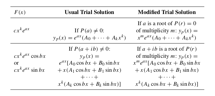
8.3: The Method of Undetermined Coefficients: Annihilators

According to Theorem 8.1.8, the general solution to the non-homogeneous differential equation
$$ P(D)y = F(x)$$
is of the form
$$ y(x) = y_c(x) + y_p(x)$$

The previous section showed how to find the solutions to $y_c$, the homogeneous linear differential equation. This section will explore how to find $y_p$, a particular solution to the non-homogeneous linear differential equation.

Insert Part about Annihilators Here

Table

Just use this table here

8.4: Complex-Valued Trial Solutions

Alternative Method for Solving the following constant coefficient differential equation
$$ y’’ + a_1 y’ + a_2 y = F(x)$$
where $$ F(x) = x^k e^{ax} \sin bx\text{ or } F(x) = x^k e^{ax} \cos bx$$

Theorem 8.4.1

If $y(x) = u(x) + iv(x)$ is a complex-valued solution to
$$ y’’ + a_1 y’ + a_2y = F(x) + iG(x)$$
then
$$ u’’ + a_1 u’ + a_2 u = F(x)\text{ and } v’’ + a_1 v’ + a_2 v = G(x)$$

Example

Find the general solution to
$$ y’’ + 9y = 5\cos (2x) $$

Note that $$F(x) = 5\cos(2x) = Re(5e^{2ix})$$

$$ z’’ + 9z = 5e^{2ix}$$
$$ z_p = z_p(x)$$

Note that
$$ y_p(x) = Re(z_p(x))$$

Since $2i$ is not a root of $r^2 + 9$, use the first row of the table to get the following
$$ z_p(x) = Ae^{2ix}$$
$$ z_p(x)’ = 2iAe^{2ix}$$
$$ z_p(x)‘‘= A(2i)^2 e^{2ix} = -4 A e^{2ix}$$

$$ -4A e^{2ix} + 9Ae^{2ix} = 5e^{2ix}$$
$$ (5A - 5)e^{2ix} = 0 \implies 5A - 5 = 0 \implies A = 1$$

So
$$ z_p(x) = e^{2ix} $$
$$y_p(x) = Re(e^{2ix}) = \cos (2x)$$

Example

$$ y’’ + y’ - 6y = 4\cos (2x) $$
Consider complex version of $F(x)$ of above
$$ z’’ + z’ - 6z = 4e^{2ix}$$
Consider homogeneous of above
$$ z’’ + z’ - 6z = 0$$
$$ (r^2 + r - 6) = (r-2)(r+3)$$
$$ r = 2, r= -3$$
$$ z(x) = c_1 e^{2x} + c_2 e^{-3x} , \ \ \ c_1, c_2 \in \mathbb{C}$$

Find $y_p$ by finding $z_p$. Note $2i$ is not a root of $(r-2)(r+3)$, so we get the following
$$ z_p(x) = Ae^{2ix} , \ \ \ A\in \mathbb{C}$$
$$ z’_p(x) =2iAe^{2ix}$$
$$ z’'_p(x) =-4e^{2ix}$$
$$ \left( -4A + 2iA - 6A \right)e^{2ix} = 4e^{2ix} $$
$$ (2i - 10) Ae^{2ix} = 4e^{2ix}$$
$$ (-5+i)A = 2$$
$$ A = -\frac{5+i}{13}$$
So
$$z_p(x) = -\frac{5+i}{13}e^{2ix} $$
$$ y_p(x) = Re(z_p(x)) = Re\left( -\frac{5+i}{13}e^{2ix} \right) = Re\left( -\frac{1}{13}(5\cos 2x - \sin 2x + i(\cos(2x) + 5\sin(2x))) \right) $$
$$ y_p(x) =-\frac{1}{13}( 5\cos_2x - \sin 2x)$$
$$ y(x) = y_c(x) + y_p(x)$$
$$ y(x) = c_1e^{2x} + c_2 e^{-3x} -\frac{1}{13}( 5\cos_2x - \sin 2x), \ \ \ \ c_1, c_2 \in \mathbb{C}$$

Example

If we wanted to solve the following
$$ y’’ + y’ - 6y = 4\sin 2x$$
we can just use the above $z_p$ value and just take the $Im(z_p)$ value since
$$ 4\sin(2x) = Im(4e^{2ix})$$

8.6: RLC Circuits

Components of Electric Circuit

• Voltage Source
  • $E(t)$
• Resistor
  • Resistance (R) measured in Ohms $\Omega$
  • Voltage Drop: $V_{drop} = IR$
• Capacitor
• Capacitance (C) measured in Farads (F)
  • Voltage Drop: $V_{drop}= \frac{q}{C}$
• Inductor
  • Inductance (L) measured in Henrys (H)
  • Voltage Drop: $V_{drop}= L \ I’(t)$

Representing the Circuit as a DE

Consider a circuit with a voltage source, one resistor, one inductor, and one capacitor
$$ IR + \frac{q}{C} + LI’ = E(t)$$

$$
I = I(t), \ \ \ \ q = q(t), \ \ \ q’(t) = I(t), \ \ \ \ I’(t) = q’'(t)
$$

$$
q’I + \frac{q}{c} + Lq’’ = E(t)
$$

$$
q’’ + \frac{R}{L}q’ + \frac{q}{LC} = \frac{E(t)}{L}
$$

The above is a 2nd order linear differential equation with constant coefficients.

$$ q(t) = q_c(t) + q_p(t)$$

If $E(t) = 0$
$$
q’’ + \frac{R}{L}q’ + \frac{q}{LC} = 0
$$
$$
r^2 + \frac{R}{L}r + \frac{1}{LC} = 0
$$

$$
r = \frac{-R\pm \sqrt{R^2 - \frac{4L}{C}} }{2L}
$$

1. Underdamped if $R^2 < 4L /C$
   $$ q_c = c_1 e^{\left( -\frac{R}{2L} + i\sqrt{\frac{4L}{C} - R^2}t \right) }+ c_2 e^{\left( -\frac{R}{2L} - i\sqrt{\frac{4L}{C} - R^2}t \right) } $$
   $$ q_c = e^{-\frac{R}{2L} t} \left( c_1 \cos \mu t + c_2 \sin \mu t \right) $$
   $$ \mu = \frac{\sqrt{\frac{4L}{C} - R^2}}{2L} $$

2. Critically Damped if $R^2 = \frac{4L}{C}$
   $$
   q_c = c_1 e^{-\frac{Rt}{2L}} + c_2 t e^{-\frac{Rt}{2L}}
   $$

3. Overdamped if $R^2 > \frac{4L}{C}$

$$
q_c = e^{-\frac{Rt}{2L}}(c_1 e^{\mu t} + c_2 e^{-\mu t})
$$

$$
\mu = \frac{\sqrt{R^2 - \frac{4L}{C}} }{2L}
$$
In all three cases, $\lim\limits_{t \to \infty} q_c(t) = 0$

So after some time, $$
q(t) = q_p(t)
$$

$q_p(t)$ is also known as the steady state charge

9.1: First-Order Linear Systems

A system of differential equations of the form is called a first-order linear system

$$ \frac{dx_1}{dt} = a_{11}(t) x_1(t) + a_{12}(t) x_2(t) + \ldots + a_{1n}(t) x_n(t) + b_1(t)$$
$$ \frac{dx_2}{dt} = a_{21}(t) x_1(t) + a_{22}(t) x_2(t) + \ldots + a_{2n}(t) x_n(t) + b_2(t)$$
$$ \vdots$$
$$ \frac{dx_n}{dt} = a_{n1}(t) x_1(t) + a_{n2}(t) x_2(t) + \ldots + a_{nn}(t) x_n(t) + b_n(t)$$

where $a_{ij}(t)$ and $b_i(t)$ are specified functions on an interval $I$

If $b_1=b_2=\ldots b_n = 0$, then the system is called homogeneous

Note that any $n$-th order linear differential equation can be replaced by an equivalent system of first-order differential equation

Example

Convert the following system of differential equations to a first-order system
$$ \frac{dx}{dt}-ty = \cos t, \ \ \ \frac{d^2y}{dt^2} - \frac{dx}{dt} + x = e^t$$

Let $x_1 = x$, $x_2 = y$, $x_3 = \frac{dy}{dt}= \frac{dx_2}{dt}$

$$ \frac{dx_1}{dt} = tx_2 + \cos t $$
$$\frac{dx_2}{dt} = x_3$$
$$ \frac{dx_3}{dt} = -x_1 + \frac{dx_1}{dt} + e^t$$
$$ \frac{dx_3}{dt} = -x_1 + \left(tx_2 + \cos t \right) + e^t$$

9.2: Vector Formulation

The following first-order system
$$ \frac{dx_1}{dt} = a_{11}(t) x_1(t) + a_{12}(t) x_2(t) + \ldots + a_{1n}(t) x_n(t) + b_1(t)$$
$$ \frac{dx_2}{dt} = a_{21}(t) x_1(t) + a_{22}(t) x_2(t) + \ldots + a_{2n}(t) x_n(t) + b_2(t)$$
$$ \vdots$$
$$ \frac{dx_n}{dt} = a_{n1}(t) x_1(t) + a_{n2}(t) x_2(t) + \ldots + a_{nn}(t) x_n(t) + b_n(t)$$
can be written as follows
$$ \vec{x’}(t) = A(t) \vec{x}(t) + \vec{b}(t)$$

$$ \vec{x}(t) = \begin{bmatrix} x_1(t) \\ x_2(t)\\ \vdots \\ x_n(t) \end{bmatrix}, \ \ \ \vec{x’}(t) = \begin{bmatrix} x_1’(t) \\ x_2’(t)\\ \vdots \\ x_n’(t) \end{bmatrix} $$
$$ A(t) = \begin{bmatrix} a_{11}(t) & a_{12}(t) & \ldots & a_{1n}(t) \\ a_{21}(t) & a_{22}(t) & \ldots &a_{2n}(t) \\ \vdots & \vdots & &\vdots \\ a_{n1}(t) & a_{n2}(t) & \ldots & a_{nn}(t) \\ \end{bmatrix}, \ \ \ \ \vec{b}(t) = \begin{bmatrix} b_1(t) \\ b_2(t) \\ \vdots \\ b_n(t) \end{bmatrix} $$

$\vec{x}$, $\vec{x’}$, $\vec{b}$ are column $n$-vector functions.

Let $V_n(I)$ be the set of all column $n$ vector functions on interval, $I$

$$ \vec{x}, \vec{x’}, \vec{b} \in V_n(I) $$

Theorem 9.2.1

$V_n(I)$ is a vector space.

Definition 9.2.2

If $\vec{x_1}(t), \vec{x_2}(t), \ldots \vec{x_n}(t)$ are all vectors in $V_n(I)$
then the Wronskian
$$ W[\vec{x_1}, \vec{x_2}, \ldots \vec{x_n}](t) = det([\vec{x_1}(t), \vec{x_2}(t), \ldots \vec{x_n}(t)]) $$

Theorem 9.2.4

If $ W[\vec{x_1}, \vec{x_2}, \ldots \vec{x_n}](t)(t_0)$ is nonzero at any point $t_0$ in $I$, the vector valued functions, $\vec{x_1}(t), \vec{x_2}(t), \ldots, \vec{x_n}(t)$ are linearly independent on $I$

Example

Show that $\vec{x_1}(t) = \begin{bmatrix} e^t \\ -e^t \end{bmatrix}$ and $\vec{x_2}(t) = \begin{bmatrix} e^t \\ e^t \end{bmatrix}$ are linearly independent.

$$ W[\vec{x_1}, \vec{x_2}] = \begin{vmatrix} e^t & e^t \\ -e^t & e^t \end{vmatrix} = 2e^{2t} \neq 0$$

9.3: General Results for First-Order Linear Differential Systems

Theorem 9.3.1

Let $A(t)$ and $\vec{b}(t)$ be continuous on $I$.
The initial value problem
$$ \vec{x’}(t) = A(t) \vec{x}(t) + \vec{b}(t), \ \ \ \vec{x}(t_0) = \vec{x_0}$$ has a unique solution on $I$

Homogeneous Vector Differential Equations

$$ \vec{x’}(t) = A(t) \vec{x}(t)$$

Theorem 9.3.2

Let $A(t)$ be an $n \cross n$ matrix continuous on $I$. The set of all solutions of the homogeneous vector differential equation $\vec{x’}(t) = A(t) \vec{x}(t)$ is a vector space of dimension $n$

• Any set of $n$ linear independent solutions to the homogeneous vector differential equation is called a fundamental solution set of $\vec{x’} = A \vec{x}$
• The corresponding matrix $X(t) = [\vec{x_1}, \vec{x_2}, \ldots, \vec{x_n}]$ is a fundamental matrix
• The fundamental solution set is just a basis of the solution space of $\vec{x’} = A \vec{x}$

Theorem 9.3.4

Let $A(t)$ be an $n \cross n$ matrix function that is continuous on $I$. If $\vec{x_1}, \vec{x_2}, \vec{x_3}, \ldots, \vec{x_n}$ is a linearly independent set of solutions to $\vec{x’} = A\vec{x}$ on $I$, then
$$ W[\vec{x_1}, \vec{x_2},\ldots, \vec{x_n}] \neq 0$$
at every point in $t$ in $I$

• This means to see if $\vec{x_1}, \vec{x_2}, \ldots, \vec{x_n}$ is a fundamental set, we only need to compute the Wronksian at one point. If $W[\vec{x_1}, \ldots, \vec{x_n}](t_0) \neq 0$, then the solutions are linearly independent (and form a basis/fundamental set), but if $W[\vec{x_1}, \ldots, \vec{x_n}](t_0) = 0$, the solutions are linearly dependent on $I$.
• The general solution to $\vec{x’} = A \vec{x}$ is just the linear combination of the elements of the basis

Proof

Show the contrapositive: If $W[\vec{x_1}, \ldots, \vec{x_n}](t_0) = 0$ at some point $t_0$ in $I$, then $\vec{x_1}, \ldots, \vec{x_n}$ is linearly dependent.

If $W[\vec{x_1}, \ldots \vec{x_n}] (t_0) = 0$ ,then $\vec{x_1}(t_0), \vec{x_2}(t_0), \ldots, \vec{x_n}(t_0)$ is linearly dependent by 4.5.17.

Then there exists $c_1, c_2, \ldots, c_n$, not all zero, such that
$$ c_1 \vec{x_1}(t_0) + c_2\vec{x_2} (t_0) + \ldots + c_n \vec{x_n}(t_0) = \vec{0}$$

Let $\vec{x}(t) = c_1 \vec{x_1}(t) + c_2\vec{x_2} (t) + \ldots + c_n \vec{x_n}(t)$. Then $\vec{x}(t)$ is the unique solution to
$$ \vec{x’} = A(t) \vec{x}(t), \ \ \ \vec{x}(t_0) = \vec{0} $$

We know that $\vec{x}(t) = \vec{0}$ is a solution to the IVP above, so by uniqueness
$$ \vec{x}(t) = c_1 \vec{x_1}(t) + c_2\vec{x_2} (t) + \ldots + c_n \vec{x_n}(t) = 0$$

But not all $ c_1, c_2, \ldots, c_n$ are zero, so $ x_1, x_2, \ldots, x_n$ are linearly dependent on $I$.

Example

$$ \vec{x’} = A\vec{x}$$
$$ A = \begin{bmatrix} 1 & 2 \\ -2 & 1 \end{bmatrix} $$
$$ \vec{x_1}(t) = \begin{bmatrix} -e^t \cos 2t \\ e^t \sin 2t \end{bmatrix}, \ \ \ \ \vec{x_2}(t) = \begin{bmatrix} e^t \sin 2t \\ e^t \cos 2t \end{bmatrix} $$

Verify that $\{x_1, x_2\}$ is a fundamental set of solutions for the vector DE and write the general solution to the vector DE

Solution

1. Find $\vec{x_1’}$ and $\vec{x_2’}$ and validate that $\vec{x_1’} = A \vec{x_1}$ and $\vec{x_2’} = A \vec{x_2}$
2. Then use the Wronksian to show that the wronskian is never zero, so $\{\vec{x_1}, \vec{x_2}\}$ is linearly independent and a fundamental set of solutions

Nonhomogeneous Vector Differential Equations

Let $A(t)$ be a matrix function that is continuous on $I$ and let $\{\vec{x_1}, \ldots, \vec{x_n}\}$ be a fundamental set on $I$ for $\vec{x’}(t) = A(t) \vec{x}(t)$. If $\vec{x_p}(t)$ is a particular solution to the nonhomogeneous vector differential equation
$$ \vec{x’}(t) = A(t) \vec{x}(t) + \vec{b}(t)$$

on $I$, then every solution to the above vector DE is of the form
$$ \vec{x}(t) = c_1\vec{x_1} + c_2\vec{x_2} + \ldots+ c_n \vec{x_n} + \vec{x_p}$$

9.4: Vector Differential Equations: Nondefective Coefficient Matrix

Theorem

If $A(t)$ is constant and diagonalizable $n\cross n$ matrix, then it is straightforward to find a basis/fundamental set for $\vec{x’} = \vec{x}$.

Let $\vec{v_1}, \vec{v_2}, \ldots, \vec{v_n}$ be $n$ linearly independent eigenvectors with $A\vec{v_j} = \lambda_j \vec{v_j}$ (eigenvectors are distinct but not necessarily eigenvalues). Then $\{e^{\lambda_1 t} \vec{v_1}, e^{\lambda_2 t} \vec{v_2}, \ldots, e^{\lambda_n t} \vec{v_n}\}$ is a fundamental set of solutions.

Proof

Since $A$ is diagonalizable, there is an invertible matrix $n \cross n$ $S$ such that
$$ S^{-1} AS = D$$
where $D$ is a diagonal matrix.

$$ A = SDS^{-1}$$
$$ \vec{x’} = \frac{d}{dt} \vec{x} = A \vec{x}$$
$$ \frac{d}{dt} \vec{x} = SDS^{-1} \vec{x}$$
$$ S^{-1}\frac{d}{dt} \left(\vec{x}\right) = D\left( S^{-1} \vec{x} \right) $$
$\frac{d}{dt}$ is a linear transformation so,
$$ \frac{d}{dt} \left(S^{-1} \vec{x}\right) = D\left( S^{-1} \vec{x} \right) $$
Let $\vec{y}(t) = S^{-1} \vec{x}(t)$
$$\frac{d}{dt} \vec{y}(t) = D \vec{y}$$
$$ y_1’ = \lambda_1y_1, y_2’ = \lambda_2 y_2,\ldots, y_n’ =\lambda_n y_n $$
$$ y_1 = c_1e^{\lambda_1t}, y_2 = c_2e^{\lambda_2t}, \ldots, y_n = c_ne^{\lambda_nt}, \ \ \ c_1, c_2, \ldots, c_n \in \mathbb{R}$$
$$ \vec{y}(t) = \begin{bmatrix} c_1e^{\lambda_1 t} \\ c_2e^{\lambda_2 t} \\ \vdots \\ c_ne^{\lambda_n t} \end{bmatrix} $$
$$ \vec{x}(t) = S\vec{y} = S\begin{bmatrix} c_1e^{\lambda_1 t} \\ c_2e^{\lambda_2 t} \\ \vdots \\ c_ne^{\lambda_n t} \end{bmatrix} $$
$$ \vec{x}(t) = \begin{bmatrix} c_1e^{\lambda_1 t} \vec{v_1} \\ c_2e^{\lambda_2 t} \vec{v_2} \\ \vdots \\ c_n e^{\lambda_n t} \vec{v_n} \end{bmatrix} $$

Example

Find a fundamental set of solutions of $\vec{x’} = A \vec{x}$
$$ A = \begin{bmatrix} -1 & 2 \\ 2 & 2 \end{bmatrix} $$

Solution

$$ \begin{vmatrix} \lambda +1 & -2 \\ -2 & \lambda - 2 \end{vmatrix} = \left( \lambda + 1 \right)\left( \lambda - 2 \right) - 4 = (\lambda - 3)(\lambda + 2) = 0 $$
Roots: $3, -2$

$$ E_3(A) = nullspace \begin{bmatrix} 4 & -2 \\ -2 & 1 \end{bmatrix} = span\left\{ \begin{bmatrix} 1 \\ 2 \end{bmatrix} \right\} $$
$$ E_{-2}(A) = nullspace \begin{bmatrix} -1 & -2 \\ -2 & -4 \end{bmatrix} = span\left\{ \begin{bmatrix} -2 \\ 1 \end{bmatrix} \right\} $$

$$ S = \begin{bmatrix} 1 & 2 \\ 2 & -1 \end{bmatrix} $$
General Solution:
$$ \vec{x}(t) = S \begin{bmatrix} c_1 e^{3t} \\ c_2e^{-2t} \end{bmatrix} $$
Fundamental Set:
$$ \left\{e^{3t} \begin{bmatrix} 1 \\ 2 \end{bmatrix}, e^{-2t} \begin{bmatrix} 2 \\ -1 \end{bmatrix} \right\}$$