notes college physics special relativity statistical physics quantum mechanics photoelectric effect compton scattering rutherford waves solid state statistical physics nuclear physics
f601fce @ 2022-12-20
7344 Words
Introduction to Modern Physics
Class Information
The course will provide an introduction to the special theory of relativity and quantum mechanics, with emphasis of their applications to atomic, molecular and solid state physics. The course is calculus based and writing intensive; it relies heavily on problem solving and technical writing.
Textbook: Modern Physics by Kenneth Krane
2: Special Relativity
Galilean Transforms
- Galilean Relativity: Also known as classical relativity. Describes how two inertial (non accelerating) reference frames see the same event (turns out to not work in all cases).
- Transforms: Allows you to convert from one coordinate frame to another
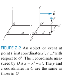
- Suppose we have two coordinate frames, $O$ and $O'$ and two different observers in each of those frames. Let $O'$ be moving away from $O$ at a velocity of $u$.
$$ x’ = x - ut$$
$$ y’ = y$$
$$ z’ = z$$
One of the postulates in Galilean Relativity, is that time is the same for all observers
$$ t’ = t$$
Visual depiction of where the $x'$ equation comes from:
Taking the derivatives with respect to time yields (note ' does not denote derivative in this case):
$$ v_x’ = v_x - u $$
$$ v_y’ = v_y$$
$$ v_z’ = v_z$$
$$ a_x’ = a_x $$
$$ a_y’ = a_y$$
$$ a_z’ = a_z$$
- Note Newton’s Laws hold in these reference frames, since acceleration are measured to be the same (as long as $u=constant$)
- Note $x, y, z$ correspond to the position of any object according to $O$, and $v_x’, v_y’, v_z'$ correspond to the velocities of an object from the perspective of $O'$
Example 2.3
Suppose a swimmer always swims with velocity $c$ relative to the water and the water relative to the river bank travels at $u$. Suppose $c > u$. Observer $O$ is on the river bank, while the $O'$ observer is traveling along the water at the same speed as $u$
Upstream and Downstream Case
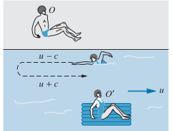
Upstream
- Note that $v_x’ = -c$ (according to observer $O'$, the swimmer moves to the left)
$$ v_x’ = v_x - u $$
$$ v_x = u - c$$ - Since $c > u$, note that $|v_x| = c - u$
- The total time to go Upstream a length $L$, is
$$ t = \frac{L}{|v_x|} = \frac{L}{c-u} $$ - Note that we use $v_x$ instead of $v_x'$, since using $v_x'$ would means some the distance traveled is actually due to the observer moving, $O'$ and not solely due to the swimmer, so the calculated time would be less than expected, and the swimmer would not actually have moved a distance $L$ according to the observer $O$ on the river bank
Downstream
- Note that $v_x’ = c$ (according to observer $O'$, the swimmer moves to the left)
$$ v_x’ = v_x - u $$
$$ v_x = u + c$$
$$ t = \frac{L}{|v_x|} = \frac{L}{c+u} $$
Calculating Time to go Upstream and then Downstream
- Just add time from upstream and downstream
$$ t = \frac{L}{c-u} + \frac{L}{c+u} = \frac{2L}{c} \frac{1}{1-u^2/c^2}$$
Cross-stream Case
We want the swimmer to swim directly across the river bank in a straight line, perpendicular from the river bank, according to observer $O$
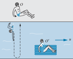
- Note that $v_x = 0$
$$ v_x’ = v_x - u \implies v_x’ = -u$$ - Note that the speed of the swimmer relative to the water is always $c$
$$c= \sqrt{v_x'^2 + v_y'^2} $$
$$ v_y’ = \sqrt{c^2 - v_x'^2} = \sqrt{c^2 - u^2}$$
$$ t=2 \cdot t_{across} = \frac{2L}{c} \frac{1}{\sqrt{1-u^2/c^2}}$$
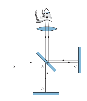
Michelson-Morley Experiment
-
Old physicists thought light had to travel in medium
- This implies preferred reference frame existed (the reference frame O’ that moved at the same speed as the medium)
- This also implied another reference frame moving at a different speed relative to the medium would have a different speed of light
-
Mirror B is half silvered (some light gets reflected while some goes through), so light travels 2 separate paths, namely AB and AC
-
There is a phase difference between the two light beams, which can be measured by looking at how many fringes appear due to interference. The phase difference is due to the following
- Difference in path length for AB and AC
- Speed of earth through ether (medium that light supposedly travels through)
-
Michelson and Morely didn’t care about 1. and wanted to measure 2. since they were trying to measure the ether
-
This is similar to Example 2.3, with $O$ being an observer on the earth and $O'$ being an observer at rest relative to ether (i.e. the preferred reference frame)
-
In order to isolate 2, they rotated the apparatus 90 degrees.
- Phase difference due to difference between AB and AC doesn’t change, since path difference doesn’t change
- But phase difference should occur due to cross-stream becoming upstream and vice versa
-
Count how many fringes change from bright to dark to see how the phase difference changes
-
Each time the fringes change, that represents a time difference between the paths due solely to movement relative to the ether and not due to the difference in path lengths of AB and AC
-
See textbook and Wikipedia for more details
Einstein’s Postulates
- The laws of physics are the same in all inertial reference frames
- The speed of light in free space has the same value in all inertial reference frames
Time Dilation and Length Contraction
- Time Dilation: Observer $O$ measures a longer time interval than $O'$
- Length Contraction: Observer $O'$ measures shorter length than observer $O$
- Proper Length $L_0$: Measured by observer where the measuring tape is at rest
- Proper time $\Delta t_0$: Measured from observer where the beginning and end of a time interval is measured at the same place
- Time dilation in one frame of reference can be seen as length contraction in another reference frame.
Simultaneity
From an observer $O$, two events could seem simultaneous, but for a different observer $O'$, these two events could seem to occur at different times.
Twin Paradox
Imagine Twin1 is on earth and Twin2 departs on a spaceship. From Twin1’s perspective, Twin2 is moving away with velocity $v$, and thus will be younger than Twin1. But from Twin1’s persepctive, Twin2 is moving away velocity $v$, so Twin1 should be yonger than Twin2. This appears to be a paradox since when Twin2 arrives back on earth, only one can be younger than the other. But in reality, Twin2 is the one accelerating/deaccelerating, and all reference frames agree Twin2 is the one doing the accelerating. Thus, Twin2 will be the one to experience the relativistic effects and be younger.
Example
Twin1 stays on earth and Twin2 departs on spaceship at age 0. Twin2 travels at $0.6c$ to a planet $6$ light years away.
- According to Twin1, it takes 6 ly/0.6c = 10 years to reach the planet and another 10 to return to earth
- According to Twin2, the length of 6 ly is contracted by a factor of $\sqrt{1 - (0.6)^2)}=0.8$. So the journey is 0.8 * 6 ly = 4.8 ly
- Since the length has been contracted for Twin2, Twin2 will measure 8 years to go to the planet and another 8 to return
- Imagine Twin1 sends a light pulse every year during the whole trip (20 years according to Twin1, 16 according to Twin2).
- The frequency at which Twin1 sends the light pulse is dopper shifted
On the journey to the planet, Twin2 will receive pulses at a frequency of
$$ 1/year \cdot \sqrt{\frac{1-u/c}{1+u/c}}=0.5/year$$
And on the journey back to earth, Twin2 will receive pulses at a frequency of
$$ 1/year \cdot \sqrt{\frac{1+u/c}{1-u/c}}=2.0/year$$ - $8 * 0.5 + 8 * 2 = 20\ pulses$
- So according to Twin2, during the 16 year journey, Twin2 receives 20 pulses, meaning Twin2 aged less
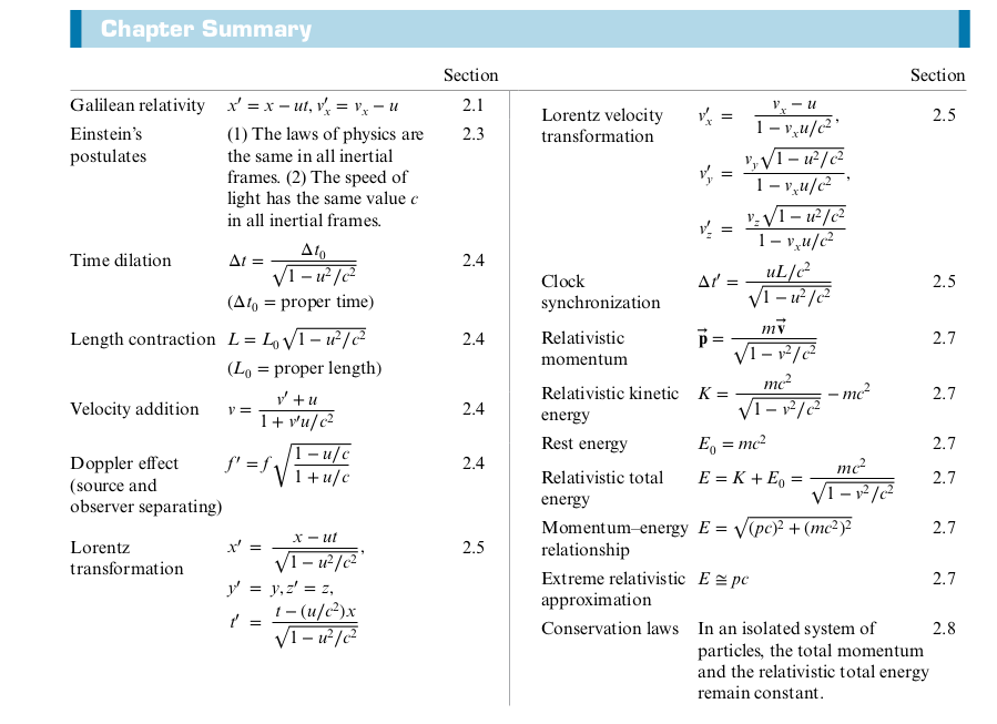
Chapter 2 Summary
Derivation in textbook:
3: Particle-Like Properties of Electromagnetic Radiation
Review of Electromagnetic Waves
$$ \vec{E} = \vec{E}_0 \sin(kz - \omega t)$$
$$ \vec{B} = \vec{B}_0 \sin(kz - \omega t)$$
- Wave Number, $k$
$$ k =2\pi/\lambda$$ - Angular Frequency ($\omega$)
$$ B_0 =\frac{E_0}{c} $$ - Pointing Vector, shows direction the EM wave propagates
$$ \vec{S} = \frac{1}{\mu_0} \vec{E} \cross \vec{B}$$
$$ P = SA = \frac{1}{\mu_0} E_0 B_0 A \sin^2 (kz-\omega t)$$
$$ P = \frac{1}{\mu_0 c} E_0^2 A \sin^2 (kz - \omega t)$$
- Note the following
- $P \propto E_0^2$
- Intensity fluctuates with time with frequency $2f = 2 (\omega/ 2 \pi)$
Diffraction
Crystal Diffraction of X Rays
-
Diffraction Grating: Device with many slits that allow us to observe interference patterns
- Superior resolution - allows separation of wavelengths close to one another
- Reasonable values of $\theta$ requires $d$ to be on the same order of magnitude as the wavelength of light being used
- Superior resolution - allows separation of wavelengths close to one another
-
Maxima corresponding to different wavelengths appear at different angles $theta$
- $d$ is the slit spacing
- $n$ is the order of the maximum ($n = 1, 2, 3, …$)
$$ d \sin \theta = n \lambda $$
X Ray Diffraction needs light on the order of $0.1$ nm in wavelength to have useful $\theta$
- This means the grating spacing has to be less than $1$ nm
- The spacing between atoms in most materials is around this value
- Use the atoms in materials as diffraction grating!
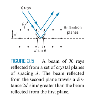
Bragg’s Law
$$ 2d \sin \theta = n \lambda$$
-
Here $\theta$ is the angle of incidence measured from the plane of the crystal
-
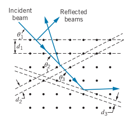
Instead of using x-ray diffraction to separate different wavelengths, we use X-Ray diffraction to see the spacing between the planes inside materials
-
We use more than one wavelength to get more $d_i$ and corresponding $\theta_i$
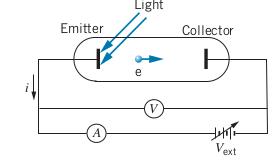
The Photoelectric Effect
- Photoelectric effect: When a metal surface is illuminated with light, it emits electrons, called photoelectrons
$$ K_{max} = eV_s$$
-
The maximum $K$ of an electron is depending on the stopping voltage $V_s$
-
The stopping voltage is determined by incrementally turning up $V_{ext}$ until the ammeter reads $0$
-
The work function ($\phi$) is the minimum energy required to remove an electron from a material
Classic Theory of Photoelectric Effect
Classical wave theory predicts the following
- $K_{max} \propto I$ since increasing the brightness of a light source increases the energy delivered to the surface and thus increases the electric field $E_0 \propto I$
- The Photoelectric effect should occur at any frequency and wavelength since according to wave theory, only the intensity of the light matters
- The first electrons should be emitted in a time interval of the order of seconds after the radiation strikes the surface
- The time interval $\Delta t$ necessary to absorb an energy of $\phi$
$$ \Delta t = \frac{\Delta E}{\Delta t} = \frac{\phi}{IA} $$
Experimental results of photoelectric effect
- For a fixed wavelength, the $K_{max}$ is totally independent of the intensity
- Doubling intensity yields no change in stopping voltage, which means the $K_{max}$ doesn’t change either
- The photoelectric effect does not occur at all if below a certain frequency
- The first photoelectrons are emitted in the order of nanoseconds
- Above results show wave theory is not enough to account for photoelectric effect
Quantum Theory of the Photoelectric Effect
-
Einstein proposed that the energy of EM radiation is not continuously distributed over the wavefront, but rather in discrete packets called photons
-
Energy of a photon
$$ E = hf = \frac{hc}{\lambda}$$ -
Einstein believed the entire energy of the photon is delivered instantaneously to a single photoelectron
- Explains why only certain frequencies work for photoelectric effect
- Explains why release of photoelectron is nearly instantaneous
-
Photoelectron is only released when the photon energy $hf$ exceeds the work function $\phi$. The excess energy appears as $K$
$$ K_{max} = hf - \phi$$ -
Intensity doesn’t appear in the above
- For a fixed frequency, doubling the intensity means twice as many photons strike the surface and twice as many photoelectrons are released, but each photon has the same $K_{max}$
-
Experiments by Millikan using the photoelectric effect were able to obtain $h$, Planck’s constant
-
Note: The value $hc = 1240 \ eV \cdot nm$ may be useful
Thermal Radiation
- Another phenomena that can’t be explained by classical wave theory
- Every object radiates thermal radiation with intensity
Stefan’s Law
$$ I = \sigma T^4$$
Wien’s Displacement Law
$$ \lambda_{max} T = 2.8978 \cross 10^{-3} \ m \cdot K$$
$$ \lambda_{max} \propto 1/T$$
-
The $\lambda_{max}$ at which the peak intensity occurs
-
Blackbody: Perfect emitter and absorber of radiation
- Whitebody Reflects all incoming radiation perfectly
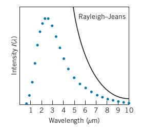
Classical Theory of Thermal Radiation
Rayleigh-Jeans Formula: Intensity per unit wavelength interval $d\lambda$
$$ I(\lambda) = \frac{2\pi c}{\lambda^4} kT$$
-
Works for long wavelengths, but fails miserably for shorter wavelengths, dubbed the ultraviolet catastrophe
-
Problem for classical physics, since E&M and Thermo, which the Rayleigh-Jeans formula was derived from, have been tested and found to be accurate, but fail for this case
Quantum Theory of Thermal Radiation
- Max Planck developed a theory where each oscillator can emit and absorb energy in discrete quantities that are integer multiples of a basic quantity of energy, $\epsilon$
$$ E_n = n \epsilon$$
$$ n = 1, 2, 3, …$$
$$ \epsilon = hf$$
This leads to a revised formula for the intensity of radiation (derivation in textbook)
$$ I(\lambda) = \frac{2 \pi h c^2}{\lambda^5}\frac{1}{e^{hc/\lambda k T} - 1}$$
- By Stefan’s Law, the following relationship between the Stefan-Boltzmann Constant and Planck’s constant can be derived
$$ \sigma = \frac{2 \pi^5 k^4}{15 c^2 h^3}$$
- Using the known value of the Stefan-Boltzmann Constant and intensity data in 1900, Planck was able to calculate the value of $h$
- 15 years later, Millikan arrived at a similar value of $h$ in a completely different experiment (Photoelectric effect), showing that the theory of quantization is a property of electromagnetic fields
The Compton Effect
-
Another way for radiation to interact with matter
-
Radiation hits electron and leads to the incoming photon and electron being scattered
-
More proof that photon exists, since the interaction implies a photon is a particle with momentum
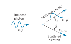
$$ \lambda’ - \lambda = \frac{h}{m_e c}(1-\cos \theta)$$
$$ \frac{1}{E_p’} - \frac{1}{E_p} = \frac{1}{m_e c^2} (1-\cos \theta) $$
$$ K_e = E_p - E_p'$$
- Compton wavelength of the Electron: Not a true wavelength but a change of wavelength
$$h/m_e c = 0.002426 \ nm$$
Bremsstrahlung
When an electron is accelerated by a potential difference $\Delta V$
$$ K_e = e\Delta V$$
An electron can hit a target and slow down, and in doing so, release the energy as bremsstrahlung (braking radiation)
In general, the energy of the photon emitted when the electron deaccelerates:
$$E_p = hf = K_e - K_e'$$
If the electron stops completely (at rest)
$$ \lambda_{min} = \frac{hc}{e\Delta V}$$
4: The Wavelike Properties of Particles
De Broglie
By this point in time, scientists knew that light had wavelike properties and had the wave-particle duality. But it was unclear whether this was only for light or whether matter could exhibit wavelike phenomena.
They knew $E = hf$ for light, but is this due to the Kinetic Energy, total energy, or relativistic energy (all the same for light)?
De Broglie hypothesized that matter can exhibit wavelike properties.
$\lambda$ is the de Broglie wavelength
$$ \lambda = \frac{h}{p}$$
- Experimental evidence like diffraction of electrons and neutrons through solids, showed that matter could actually exhibit wavelike properties
Heisenberg Uncertainty Relationships
$$\Delta x \Delta p_x \ge \frac{1}{2} \hbar $$
- $\Delta x$ is uncertainty in position
- $\Delta p$ is uncertainty in momentum
$$\hbar = \frac{h}{2\pi}$$
$$\Delta E \Delta t \ge \frac{1}{2} \hbar $$
6: The Rutherford-Bohr Model of the Atom
Franck-Hertz Experiment
-
Direct evidence that electrons in atoms can exist in discrete excited states
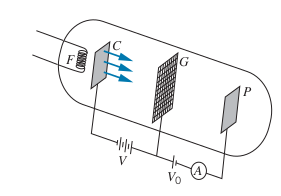
The Filament, $F$, is heated and emits electrons. There is a voltage $V$ between $C$ and $G$, that accelerates the electrons towards the grid, $G$. In the tube is a gas such as mercury. There is a retarding voltage $V_0$ that only allows the electrons to reach $P$ if $V > V_0$. The ammeter measures the current from electrons reaching $P$.
- As $V$ increases, more electrons have enough KE to get to $P$. Whenever an electron collides with a mercury atom, energy is conserved (perfectly elastic).
- Then at a certain $V$, ($4.9$ for mercury), all collision with mercury atoms are perfectly inelastic, and all the energy from the electron goes into raising the mercury atom’s electrons to the first energy level. So less electrons have enough KE to reach the $P$, so current drops.
- Repeat 1. and 2.
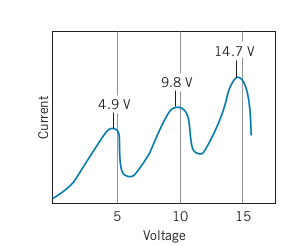
-
Every time there is a drop in current, the voltage at the peak current is a multiple of 4.9
-
Also note that the distance between the peaks is 4.9
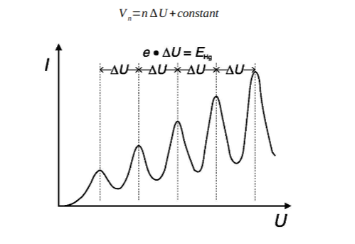
-
$V_n$ is the $V$ at the peak
Rutherford Scattering Experiment
Juicy derivation in textbook
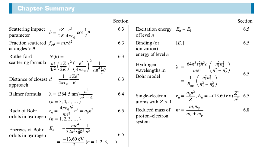
Summary
5: The Schrödinger Equation
Schrödinger Equation describes the electron (or any other quantum state) as a wave. Using the wave function, we can find the average momentum, average position, and the probability of finding the particle in certain positions.
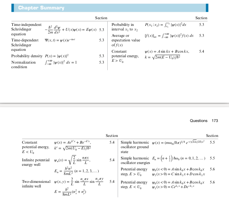
Summary
Two-Dimensional Quantum Oscillator
$$ E = \frac{h^2}{8mL^2}(n_x^2 + n^2_y)$$
- Note that if there are two ways for $E=13E_0$
- $n_x = 3, n_y = 2$
- $n_x = 2, n_y = 3$
- There are three ways for $E=50E_0$
- $n_x = 7, n_y = 1$
- $n_x = 1, n_y = 7$
- $n_x = 5, n_y = 5$
- The number of ways for a system to be at a certain energy is called the degeneracy
- $E=50E_0$ has a degeneracy of 3, and $E=13E_0$ has a degeneracy of 2
- Degeneracy arises from more than one quantum number
- The number of quantum numbers describing a system is equal to the number of dimensions (e.g. 2 quantum numbers for 2D problem)
- Degeneracy gives rise to a lot of the properties and structure of atoms
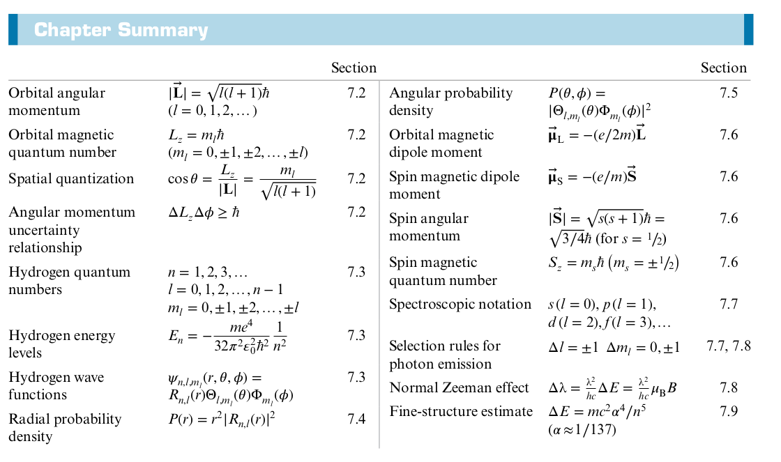
7. The Hydrogen Atom In Wave Mechanics
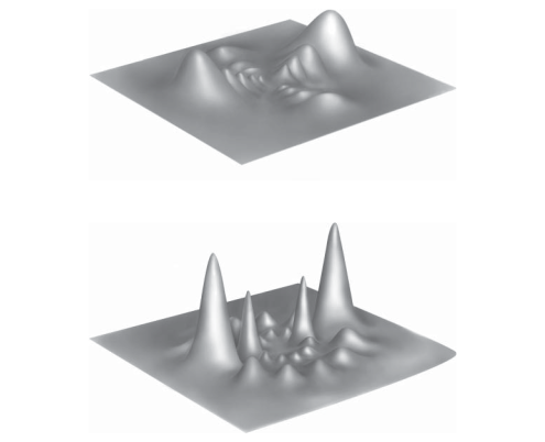
Above shows the probability of finding an electron in $n=8$ with angular momentum $l=2$ (top) and $l=6$ (bottom) in the xz plane, with the height of the peaks corresponding to the probability.
Deficiencies in Bohr-Rutherford Model
- Looking at spectral lines showed two streaks close to each other, not addressed by Bohr Model
- Later found to be due to intrinsic spin of electron
- The Bohr Model has the electron in an orbit around the nucleus at a fixed radius
One Dimensional Atom
$$ U(x) = -\frac{e^2}{4\pi \epsilon_0 x}$$
We can use the Schrödinger Equation to solve the above Coloumb potential in one dimension
$$ -\frac{\hbar}{2m} \frac{d^2 \psi}{dx^2} - \frac{e^2}{4\pi \epsilon_0 x} \psi(x) = E \psi(x) $$
A trial solution for the above differential equation:
$$ \psi (x) = Ax e^{-bx}$$
Substituting the trial solution gives
$$ b = \frac{me^2}{4\pi \epsilon_0 \hbar^2} = \frac{1}{a_0} $$
where $a_0$ is the Bohr radius
Angular Momentum in the Hydrogen Atom
-
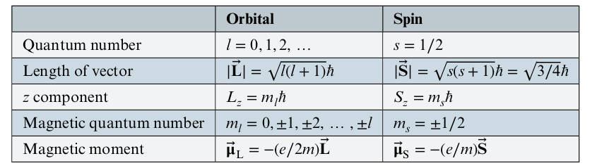
Bohr’s model treated angular momentum as quantized, with the angular momentum of an electron as $|\vec{L} | = n\hbar, \ \ n = 1, 2, 3, …$
-
But the quantum version of angular momentum
$$ |\vec{L}| = \sqrt{l(l+1)} \hbar , \ \ \ l = 0, 1, 2, 3,… $$ -
$m_l$, the magnetic quantum number, describes the angular momentum for one component
$$ L_z = m_l \hbar, \ \ \ m_l =0, \pm 1, \pm 2, … \pm l$$ -
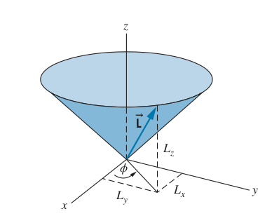
We can only know at most one component of $L$ and $|\vec{L}|$, that is we can only know $l$ and $m_l$. Since a vector has to be described by at least 3 number, there is some incomplete information about the angular momentum vector. Thus we will never know the other two components of the angular momentum
-
If we know $L_z$, we can’t know $L_y$ or $L_x$, which is equivalent to
$$ \Delta L_z \Delta \phi \ge \hbar$$
Graphical Representation of the uncertainty for angular momentum
The Hydrogen Atom Wave Function
We can represent the wave function in 3D in spherical coordinates
$$ \frac{\hbar^2}{2m} [\pdv[2]{\psi}{r} + \frac{2}{r} \pdv{\psi}{r} + \frac{1}{r^2 \sin \theta} \pdv{\theta} \left(\sin \theta \pdv{\psi}{\theta}\right) + \frac{1}{r^2 \sin^2 \theta} \pdv[2]{\psi}{\phi}] + U(r) \psi(r, \theta, \phi = E \psi (r, \theta, \phi)$$
The potential energy only depends on $r$ since the Colomb potential only depends on $r$, so the wave function that solves the above is of the following form
$$ \psi (r, \theta, \phi) = R(r) \Theta (\theta) \Phi(\phi)$$
- Radial Function $R(r)$
- Polar Function $\Theta (\theta)$
- Azimuthal Function $\Phi(\phi)$
Each function is a function of a single variable
$$ \psi_{n, l, m_l} (r, \theta, \phi) = R_{n, l}(r) \Theta_{l, m_l} (\theta) \Phi_{m_l}(\phi)$$
Quantum Numbers
Since the hydrogen wave function is 3D, we have 3 quantum numbers:
- $n$, principle quantum number: corresponds to the energy level of an electron, $1, 2, 3, …$
- $l$, angular momentum quantum number: $0, 1, 2, 3, …, n-1$
- $m_l$, magnetic quantum number: $0, \pm 1, \pm 2, …, \pm l$
Recall that $n$ determines the energy level
* At $n=1$, the degeneracy is 1 (number of possible quantum number combinations)
* At $n=2$, the degeneracy is 4
* At $n=3$, the degeneracy is 9
* In general, at energy $E_n$, the degeneracy is $n^2$
- You can find the probability density by integrating $|\psi_{n, l, m_l}(r, \theta,\phi)|^2 dV$
Intrinsic Spin (Stern-Gerlach Experiment)
An orbiting electron creates a magnetic dipole moment in an external magnetic field, which allow counting $l$ and observing a component of $\vec{L}$
-
The Stern-Gerlach experiment had a non-uniform magnetic field cause an uneven force applied to the incoming atoms to move to one direction or another
- The atoms went to specific spots on the target screen, showing quantization
- Three spots, center (no deflection, up, and down)
- However each of these three spots was actually composed of two more sub subspots, indicating the electron itself also had a spin
- Electron’s intrinsic spin arises from relativistic effects
Energy Levels and Spectroscopic Notation
Selection Rule
When an electron loses energy and goes to a lower state, the selection rule shows the most probable transitions, obtained by solving Schrödinger’s equation and computing transition probabilities
$$ \Delta l = \pm 1$$
Examples:
- 3s cannot emit photon in 2s ($\Delta l = 0$) and instead goes to 2p $\Delta l = 1$)
- 3p can go to 2s or 1s, but not $2p$
Summary
8: Many-Electron Atoms
- Orbit of earth around sun
- Simplify by only considering two body problem
- Good approximation since other planet’s gravity is miniscule compared to sun’s
- Electrons and Nucleus
- Can’t approximate like in the above problem when dealing with more than one electron around the nucleus
- Each electron exerts a force on every other electron around the nucleus
- This force is significant, so you can’t just correct for it and only consider the force from nucleus
- Example of Many-body problem, with 3 or more particles mutually interacting with each other
Pauli Exclusion Principle
- We might think that all the electrons will occupy the lowest energy level, which is the 1s state
- But if this were true, the properties of atoms would vary smoothly
- Most properties of different elements don’t vary smoothly, with the exception of the energy of x-rays emitted by atoms
- But if this were true, the properties of atoms would vary smoothly
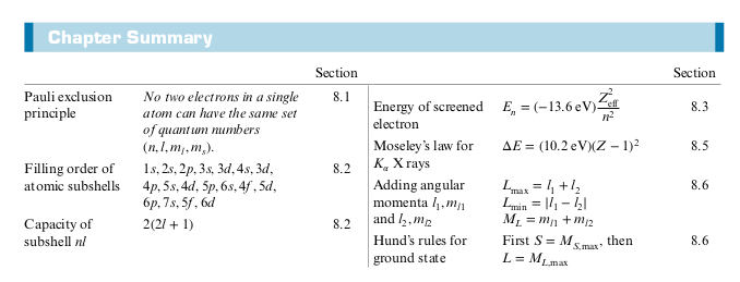
- Pauli Exclusion Principle: No two electrons in a single atom can have the same set of quantum numbers ($n$, $l$, $m_l$ , $m_s$).
Electronic Structure of Many-Electron Atoms
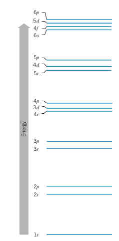
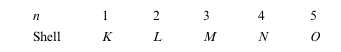
- Electrons in the same shell (same $n$) have the same average distance from the nucleus
- Subshells: Specific combinations of $n$ and $l$
- E.g. 3s, 4p, 3d, 2s, etc.
- Total number of electrons with in a subshell is $2(2l + 1)$
- 2 factor comes from two spin $m_s$ values, and the $2l+1$ comes from possible values for $m_l$ for a given $l$
Outer Electrons: Screening and Optical Transitions
- Electron Screening: Electrons in the outer levels experience less of the charge from the nuclues due to the repulsive forces from the electrson in inner shells. Thus the effective charged experienced by the outer electrons is less
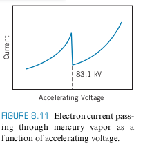
Inner Electrons: Absorption Edges and X-Rays
-
If we repeat the Franck Hertz Experiment but with tens of kV instead of tens of volts, we can knock out the inner electrons instead of the outer electrons
-
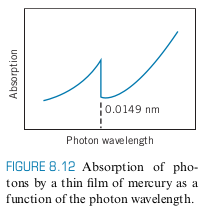
We get the following graph if we perform FH experiment on Hg with kV
- 83.1 kV corresponds to 0.0149 nm, which is in the X-ray region
- 83.1 kV corresponds to 0.0149 nm, which is in the X-ray region
-
If we bombard a thin film of mercury with x-rays, we see the absorption drops at 0.0149 nm (photoelectric effect), in agreement with above experiment
- Absorption Edge: Sudden drop in current or absorption
- Absorption Edge: Sudden drop in current or absorption
-
K corresponds to $n=1$, so the K Absorption Edge is the absorption edge for when the innermost electron
X-Ray Transitions
- We showed previously, that one way to produce x-rays is through Bremsstrahlung by accelerating electrons and then slowing them down
- This produces a continous x-ray spectrum
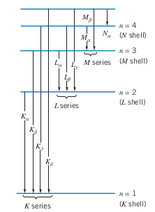
- One way to produce discrete x-ray spectrum is by allowing an inner electron to move down to a lower energy level
- E.g. knock out 1s electron. This leaves vacancy in K shell, so another electron from another shell $L, M, N, …$ comes to fill the K vacancy
- If an electron from the $L$ shell comes to fill the $K$ vacancy, the X-ray created is a $K_\alpha$ X-ray
- If an electron from the $M$ shell comes to fill the $K$ vacancy, the X-ray created is a $K_\beta$ X-ray
Moseley’s Law
The energy for a $K_\alpha$ X-ray is related to the atomic number of the element $Z$
$$ \Delta E = (10.2 \ eV ) (Z- 1)^2 $$
Chapter 8 Summary
9: Molecular Structure
Chapter 9 Summary
10: Statistical Mechanics
- Some experiments can be described by looking at single isolated events
- Rutherford Scattering
- Compton Scattering
- But for many phenomena, you have to analyze the average behavior using statistics
- Classical Statistics
- Quantum Statistics
Statistical Analysis
- Microscopic properties
- Velocity and Position of every single atom
- Not practical for even a small system containing $10^{15}$ atoms
- Macroscopic properties
- Temperature and pressure of a gas
- Relationship between microscopic and macoscopic properties
Macro/Micro state Example
Consider a system with 4 particles with a maximum allowed energy of 2 units of energy
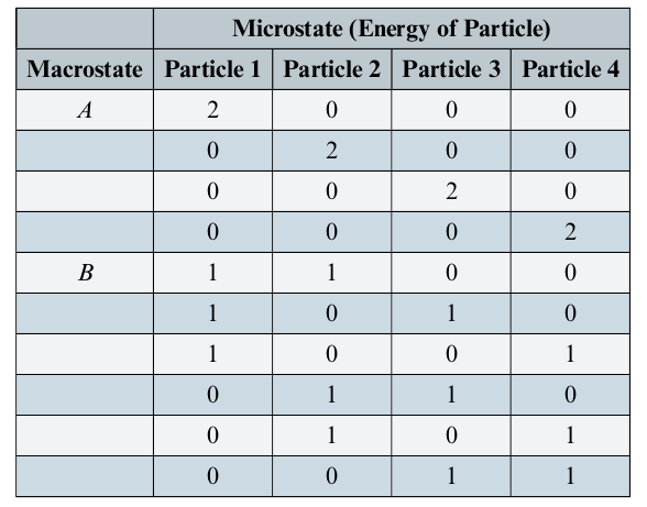
- Macrostate
- A: Only one particles has 2E
- B: Two particles have 2E
- Microstate
- Total of 10 microstates (with 40 particles total)
- The number of microstates for a particular macrostate is called the multiplicity and denoted with $W_{macrostate}$
- $W_A = 4$ means macrostate A has 4 microstates
- $W_B = 6$ means macrostate B has 6 microstates
- All microstates of a system are equally probable
- E.g. In this example, the probability of finding a system in macrostate B 60% of the time
- Probability of finidng a particle with 2E is 4/40 = 10%
Classical and Quantum Statistics
Consider a system with 6 units of energy total and with 5 identical particles
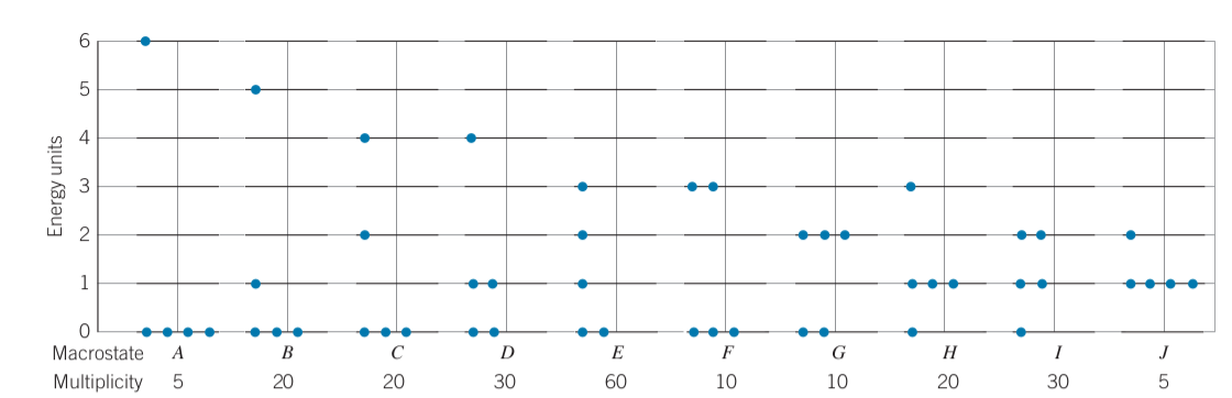
-
Multiplicity of each macrostate (Number of microstates per macrostate):
$$W= \frac{N!}{N_0! N_1! N_2! N_3! N_4! N_5! N_6!} $$- Where $N$ is the total particles and $N_E$ is the number of particles at energy E
-
Total number of microstates for $N$ distinguishable particles sharing $Q$ units of energy
$$ W_{total} = \frac{(N+Q-1)!}{Q! (N-1)!}$$ -
Probability of finding a particle with energy, $E$
$$ p(E) = \frac{\sum\limits_i N_i W_i}{N\sum\limits_i W_i}$$- Where $N_i$ is the number of particles with energy E in each particular macrostate
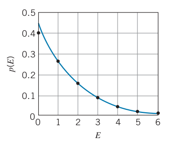
- The curve shows $p \propto e^{-\beta E}$ which turns out to be correct
- Some other phenomena do not behave as well with classical physics such as electric conductivity, heap capacity
Quantum Statistics
- Quantum particles must be treated as indistinguisable
- Multiplicity of each macrostate is 1
- Quantum mechanics imposes limits on max number of particles in a given state
- E.g. electrons have spin up or down, no two electrons in the same state
The Density of States
-
Distribution Function: $f(E)$ Gives probability of finding particle of energy $E$
-
Our ultimate goal is to find a function that gives us the number of particles at energy $E$
- This quantity depends on $f(E)$ but also how many states are available at a given energy $E$
- The number of states available at energy $E$ is just the degeneracy, $d_n$
- Example: For dilute hydrogen gas, the number of states available at each energy level, $E_n$, is the degeneracy which is $2n^2$ for a state with principle quantum number, $n$
- Example: For a molecule with rotational excited states like HCL, the number of states available at each energy level, $E_L$, is the degeneracy which is $2L+1$ for a state with angular momentum number $L$ (See Chapter 9)
- The number of states available at energy $E$ is just the degeneracy, $d_n$
- This quantity depends on $f(E)$ but also how many states are available at a given energy $E$
-
Thus we have the following expression for the number of particles at a given $E_n$
$$ N_n = d_n f(E_n) $$- where $N_n$ is the number of particles at a given $E_n$
$$ N = \sum N_n = \sum d_n f(E_n)$$
- where $N_n$ is the number of particles at a given $E_n$
-
$N$: total number of particles
-
For large systems, we can’t keep track of every individual particle and separate out each individual state, so we look at the number of states in a small interval $dE$ at energy $E$ (equivalently, the number of states between $E$ and $E+dE$)
- treats $E$ as continuous
-
The Density of States $g(E)$ is defined so that $g(E) dE$ is the number of available states per unit volume between $E$ and $E+dE$ (or equivalently in $dE$ at energy $E$)
-
The number of populated states, $dN$ in the interval $E$ to $E+dE$ is as follows
$$ dN = N(E) dE = V g(E) f(E) dE$$
$$ N = \int dN = \int_0^\infty N(E) dE = V \int_0^\infty g(E) f(E) dE $$ -
$N(E)$: number of particles per unit energy interval at a particular energy E (has units of $\text{energy}^{-1}$)
Density of States of Gas of Particles (Electrons or Molecules)
$$ g(E) = \frac{4\pi(2s+1)\sqrt{2} (mc^2)^{3/2}}{(hc)^3} E^{1/2}$$
where $s$ is the spin
- Derivation in textbook
Density of States in a Gas of Photons
$$ g(E) = \frac{8\pi}{(hc)^3} E^2$$
- Derivation in textbook
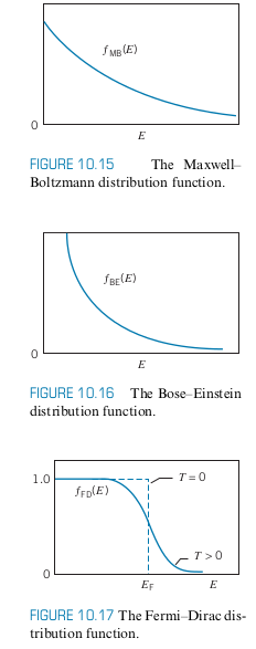
Quantum Statistics
-
Particles that don’t obey Pauli Exclusion principle have integer spins $0, 1, 2, …$ in units of $\bar h$ and are called Bosons
- Their properties are determined by the Bose-Einstein Distribution Function
$$ f_{BE}(E) = \frac{1}{A_{BE}e^{E/kT} - 1}$$- where $A_{BE}$ is a normalization constant that remains pretty constant with respect to $T$
- Their properties are determined by the Bose-Einstein Distribution Function
-
Particles that do obey Pauli Exclusion principle have half integer spins $1/2, 3/2, …$ in units of $\bar h$ and are called Fermions
- Their properties are determined by the Fermi-Dirac Distribution Function
$$ f_{FD}(E) = \frac{1}{A_{FD}e^{E/kT} + 1}$$- where $A_{FD}=e^{-E_F/kT}$ is a normalization constant that depends on $T$
$$ f_{FD}(E) = \frac{1}{e^{(E-E_F)/kT} + 1}$$ - $E_F$ is the Fermi Energy
- where $A_{FD}=e^{-E_F/kT}$ is a normalization constant that depends on $T$
- Their properties are determined by the Fermi-Dirac Distribution Function
-
Suppose the normalization constants are $1$
-
For small $T$, $f_{BE} \to \infty$, so all the bosons try to occupy the lowest energy state (Boson Einstein Condensation)
-
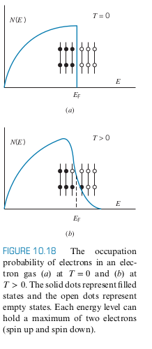
For small $T$, not all the fermions can occupy the same state due to the Pauli Exclusion Principle. When $E<E_F$, $f_{FD} \to 1$ and for $E>E_F$, $f_{FD} \to 0$. When $E=E_F$, $f_{FD} = 0.5$ (like the logistics function)
- Consider a gas of electrons with $g(E)$ and $f_{FD}$. $N(E) = V g(E) f_{FD}(E)$
- The figure below shows a possible configuration of electrons
- Notice that only the states near $E_F$ are affected by an increase in temperature. The states at very low energies stay filled while the states at very high energies remain unfilled
Limits of Classical Statistics
-
Quantum behaviour can be neglected when $\lambda_{Broglie} \ll d$, where $d$ is the separation between the particles (i.e. no particle lies within the wave packets of its neighbors)
-
Thus we can still use classical statistics whenever $\lambda \ll d$ or $\lambda/d \ll 1$
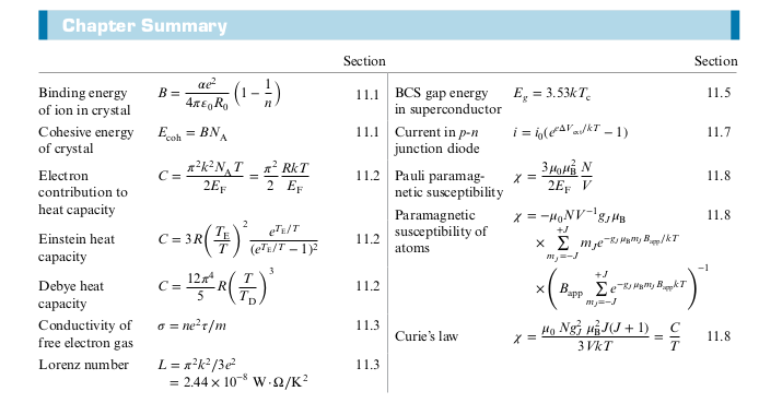
Chapter 10 Summary
11: Solid State Physics
- Properties of solids based on quantum mechanical interactions
- Solid State Physics is often called Condensed Matter Physics nowadays
Crystal Structures
- Crystal: Atoms/Molecules occupy places in a latice at periodic intervals
- Salt, Metals, etc.
- Long-Range order: We can determine how the crystal looks by looking at a local arrangement of molecules/atoms, due to the repeating nature of the lattice
- Amorphous Solid: No repeating pattern/structure
- Glass, Paper
Ionic Solid
-
Coulomb Force
-
Cubic Lattice
-
Face Centered Cubic (FCC)
-
Body Centered Cubic (BCC)
-
Adding up the individual Coulomb potential energies from every other atom yields a convergent infinite series
Covalent Solid
Metalic Solid
- D orbitals form a “sea of electrons” (Fermi-Gas)
Molecular Solid
- Depends on Dipole Bonds (e.g. hydrogen bonds)
- Note how much weaker bonds in molecular solids are
- Coulomb force $\propto \frac{1}{R^2}$
- Dipole $\propto \frac{1}{R^3}$
Heat Capacity of Solids
Classical thermodynamics
- The equipartiaion theorem states each degree of freedom has $\frac{1}{2} kT$ energy
- 6 degrees of freedom for particle in a lattice
- Expect there to be $\frac{6}{2}kT = 3kT$ energy per atom in a lattice
- Heat Capacity, $C$ is just $\frac{dE}{dT}$
- $\implies C = \frac{d(\frac{1}{2}kT)}{T} = 3k$
- This would mean that the heat capacity for all solids is the same at all temperatures
- Result is known as Law of Dulong and Petit
- Works well at room temperature, but not as temperature is decreased
- Result is known as Law of Dulong and Petit
Apply Quantum Statistics
- Assume heat capacity is due to electrons in metal (Fermi Gas)
- $kT \ll E_F$
We get the following result
$$ C = \frac{\pi^2}{2} \frac{RkT}{E_f} $$
- The above results predicts that the graph of $C vs. T$ is linear, however, this is not the case
- Copper’s heat capacity at $C$ is much higher than predicted by above, indicating the contribution by electrons is smaller than expected
Einstein’s Theory
- Assumed oscillations of the solid (not atom) obey Bose-Einstein statistics
- EM quanta (i.e. photons) obey Bose-Einstein statistics
- Similarly, phonons quanta of vibrational energy obey Bose-Einstein stats
- Assume that all phonons have same vibrational frequency
Quantized oscillator
$$ E = (n+\frac{1}{2}) \bar h \omega$$
- $N_A$ atoms/mol
- $3N_A$ oscillations/mol
Boson gas
$$ E_{int} = 3N_A f_{BE} = \frac{3N_A}{e^{-\bar h \omega/ kT } - 1}$$
$$ C = \frac{dE}{dT} = 3R(\frac{T_E}{T})^2\frac{e^{T_E/T}}{(e^{T_E/T}-1)^2}, \ \ T_E = \frac{\bar h}{K}$$
-
$T_E$ is the Einstein temperature
-
Peter Debye: Then expanded on above, and assumed phonons have a continous spectrum of frequencies (like photons) instead of discrete frequencies
$$ C = \frac{12\pi^4}{5}(\frac{T}{T_D})$$ -
$T_D$ is the Debye temperature
-
The total heat capacity is a combination of the Bosonic lattice vibrations and the Fermic Gas electron contributions
$$ C = aT + bT^3$$ -
The $aT$ term (electron contribution) has a greater effect at very low temperatures since the $T^3$ term goes rapidly to zero
Electrons in Metals
Electrons can be treated as fermi gas
$$ N = \int_0^\infty N(E) dE = \frac{8\sqrt{2}\pi Vm^{3/2}}{h^3} \int_0^\infty \frac{E^{1/2} dE}{e^{(E-E_F)/kT} + 1}$$
$$ \implies E_F(T) \approx E_F(0) \left[1- \frac{\pi^2}{12}\left(\frac{kT}{E_F(0)}\right)^2\right]$$
- Even though the Fermi energy depends on temperature, we can assume it is constant for a material since the Fermi energy at 0K and room temperature is pretty much the same
Electric Conduction
$$ \vec{j} = \sigma \vec{E}$$
where $j$ is the current density, the current per unit cross-sectional area, $E$ is the electric field applied to the metal, and $\sigma$ is the conductivity of the metal
- Assume current is constant in conductor
- When electrons are accelerated by $\vec{E}$, they collide with atoms in lattice and are slowed down
$$ \vec{F} = m\vec{a}= -e \vec{E}$$
$$ \implies \vec{a} = \frac{-e\vec{E}}{m} $$ - Electrons acquire on average a drift velocity $\vec{v_d}$ every time it is accelerated equal to acceleration times time, $\tau$
$$ \vec{v_d} = \frac{-e\vec{E}}{m} \tau$$
- When electrons are accelerated by $\vec{E}$, they collide with atoms in lattice and are slowed down
- We also have $\vec{j}$ proportional to $n$, the density of electrons in the conductor
$$ \vec{j} = -n e \vec{v}_d$$ - Combinbing gives
$$ \vec{j} = \frac{ne^2 \tau}{m}\vec{E}, \ \ \sigma = \frac{ne^2\tau}{m}$$
$$ \tau = \frac{l}{v_{avg}}$$- $l$ is the mean free path (average distance electrons travel before colliding with atoms)
- $v_{avg}\neq v_{D}$ since $v_{avg}$ is the average velocity the electrons travel through the lattice while $v_d$ is the small increase in speed that comes from $\vec{E}$
For a classical particle
$$ K = \frac{3}{2}kT$$
- If we take $l$ to be the spacing between the lattice and treat the electrons semi-clasically, this gives $\sigma \propto T^{-1/2}$, however experimental data shows $\sigma \propto T^{-1}$
Quantum Theory of Electrical Conduction
- Treating the electrons as a fermi gas instead of a classical particle with velocity $v_F$ yields an even worse value for $\sigma$
- Thus that means our $l$ assumption should be updated
- A perfect lattice means the mean free path is infinite and thus $\sigma$ is infinite
- A perfect lattice means a infinite conductivity
- In a real metal lattice, the following contribute to electron scattering
- Atoms are in random thermal motion, so the lattice is not always perfect
- Dominates at high temperatures, depends on $T$
- Lattice imperfections/impurities
- Dominates at lower temperatures, independent of $T$
- For thermal motion: Average vibrational potential energy is proportional to $T$, agreeing with measurements
- Thermal conductivity behaves in almost the same way as electrical conductivity
- The ratio of thermal conductivity and electrical conductivity is independent of material, but depends on temperature, since $kT$ determines number of electrons available for thermal conduction
- Wiedemann-Franz Law
$$ \frac{K}{\sigma T} \approx L = \pi^2k^2/3e^2 $$
where $K$ is the thermal conductivity and $L$ is the Lorenz number- Not always correct since it assumes $l$ is the same for thermal and electrical conductivity See wikipedia for derivation
Band Theory of Solids
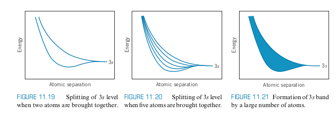
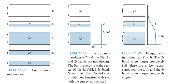
- Consider Sodium with a half-filled 3s subshell
- When we move more an more sodium atoms together, the wavefunctions overlap. When we have a very large number $\approx 10^{22}$ or more, there is a solid band that forms, since the individual wavefunctions are no longer distinguishable
- Each band can hold $2(2l+1)N$ electrons, where $N$ is the number of atoms
-
Notice that $E_F$ is located halfway in the 3s band
- 3s is the conduction band
- Even a small potential (~1V), electrons can absorb energy since there are $N$ unoccupied states in the 3s band all within an energy of $1 \ eV$ of each other
-
At the ground state, Sodium’s 3s band holds $N$ electrons and when $T=0$
-
Consider all the other bands in sodium
-
Conductors have the Fermi level halfway within a band
- There are $N$ free electrons that can move to $N$ unoccupied states
-
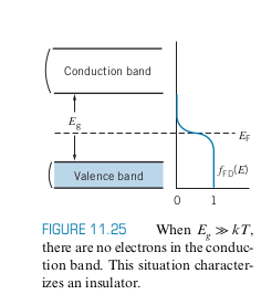
Insulators have the Fermi level halfway between two different bands (See below) and a large gap with $E_{g} \gg kT$, wher $E_g$ is the gap energy
- Even when the FD distribution spreads out when $T$ increases, the spread is not large enough to bridge the gap between the Valence Band and the conduction Band
- Even though there are a large number of electrons in the valence band for electrical conduction, there are not many unoccupied states they can move to, so there is no way they contribute to conduction
- Although the conduction band has lots of empty states, there are almost no electrons in the conduction band to contribute
-
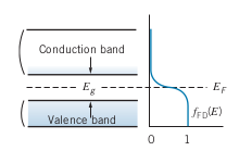
Semiconductor: Similar band structure as insulators, but with the gap energy at around $1 \ eV$
- A small population of electrons can occupy a bit of the conduction band
- Below is an example of the band structure at room temperature. Note the lighter blue indicates that there are a few electrons in the conduction band with lots of unoccupied states to move to, and there are a lot of electrons in the valence band with a few unoccupied states to move to as well, which both contribute to a bit ofconduction
- The conductivity of semiconductors also depends more on the temperature as well, since increasing temperature spreads out the $f_{FD}$ function, meaning more conduction
- Doping, which involves introducing small amounts of impurities, can also move the $E_F$ around, affecting conductivity
Superconductivity
-
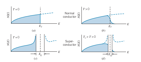
For an ordinary conductor, as $T$ approaches $0$, the contribution to resistance from impurities in the lattice remains constant, so the resistance approaches a constant value
-
However, for a supercondcutor, the resistance rapidly goes to 0 below a certain $T_C$, called the cricial temperarture
-
BCS theory states that as temperature is decreased for a superconductor, there is an energy gap, $E_g$ that widens
- At and below $T_C$ Cooper pairs form to the left of the energy gap, where the pairs are electrons that behave as non-fermions (meaning the population can exceed limits of the FD distribution)
- The energy gap represents the binding energy of the cooper pairs
$$ E_g = 3.53 kT_C$$
Intrinsic and Impurity Semiconductors
-
$E-E_F = 0.5 \ eV$ if $E_F$ is in the middle of a gap of $E_G = 1 \ eV$, $kT ~ 0.025 \ eV$ at room temperature, so $e^{-E_g/2kT} \approx 10^{-9}$
-
There is one atom in $10^9$ contributes to conduction in a semiconductor
-
Thus if there are $10^{20}$ atoms in a material, there around $10^{11}$ conduction electrons in a semiconductor, $10^{20}$ in a conductor, and none in an insulator
-
Holes exist in the valence band if some electrons are in the conduction band
- Conduction in an intrinsic semiconductor is due to the electrons moving in the conduction band and also due to the positively charged holes “moving”
- Electrons move more easily, so contribute more than holes to conduction
-
Doping creates impurity semiconductors
- N-Type: Uses Donor atoms that donate electrons to the conduction band
- Phosphorus, arsenic, etc.
- P-Type: Uses acceptor atoms that add holes to the valence band
- Boron, Gallium, etc.
- Adding donors or acceptors creates new energy bands/states
- At $T=0$, the donor states are all filled and the acceptor states are all empty (recall that at $T=0$, all bands below $E_F$ are filled and all below are empty)
- As $T$ increases, $E_F$ starts moving towards the middle of the gap
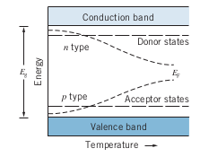
- N-Type: Uses Donor atoms that donate electrons to the conduction band
Semiconductor Devices
Diode
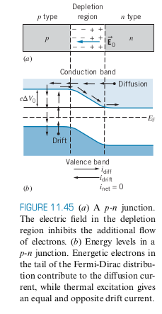
- When a P-type semiconductor and N-Type semiconductor are placed in contact with one another, electrons move from the n-type to the p-type
- In the middle of the two is the depletion region, where charge carriers are somewhat depleted, since the holes are already filled with electrons from the n-type
- Excess electrons that have filled holes in p-type give it a negative charge and the lack of electrons in the n-type give it a positive charge
- At equilibrium, there is enough negative charge in the p region to repel more electrons. At equilibrium, $E_F$ is the same for both p region and n region as well.
- At equilibrium there is a potential $\Delta V_0$, so there is an energy barrier $e\Delta V_0$
- Drift Current and Diffusion Current: equal at equilibrium
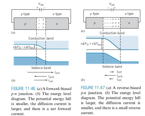
- When you apply a voltage, the energy barrier is raised or lowered, and affects the drift and diffusion currents, so that they are no longer equal
- Reverse Bias: Causes very little current to flow
- Forward Bias: Causes a significant amount of current to flow
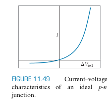
- Note how current basically only flows through one way: Diode
Photodiode
- External current excites electron from valence to conduction, when the electron drops, light is emitted
- Note that the energy gap is on the order of $1 \ eV$ which is perfect since visible light is on the order of $2 \ eV$ to $3 \ eV$
- Running the photodiode in reverse can be used to count photons or used as a solar cell type thing
Chapter 11 Summary
12: Nuclear Structure and Radioactivity
Nuclear Constituents
Nuclear Size and Shape
Nuclear Mass and Binding Energies
The Nuclear Force
Quantum States in Nuclei
Radioactive Decay
Alpha Decay
Beta Decay
Gamma Decay and Nuclear Excited States
Natural Radioactivity
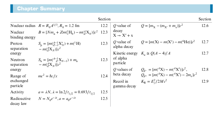
Chapter 12 Summary
13: Nuclear Reactions and Applications
Experimental Techniques in Nuclear Physics
- In nuclear physics, the energy range is in MeV or more
- Simple method
- Hold two plates with a potential difference
- Cons: Huge potential between the two plates
- Hold two plates with a potential difference
- Linear Accelerator (LINAC)
- Oscillating polarities for tubes
- Longer and longer tubes as you go down
- Largest: Stanford Linear Accelerator (SLAC)
- Cyclotron
- Two Half shells called Dees
- Magnetic Field used to make particles accelerate in a circular orbit
- As time passes, the particles reach larger and larger energies, so the orbits gets larger and larger
- Modern Particle Accelerator
- Two beams circling around in opposite directions
- Larger and larger energies mean uncertainty in energy get larger and larger
- Increases probability of more massive particles like the Higgs Boson
Types of Nuclear Reactions
Nuclear Reactions can be represented as follows
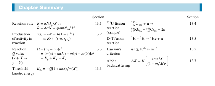
$$ x + X \rightarrow y + Y$$
- If there is no external force, then energy, momentum, and angular momentum are all conserved
Nuclear Fusion
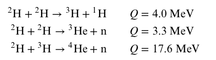
- Notice that the deuterium-tritium (DT) reaction releases the most energy
- $n$: Density of plasma
- $T$: Temperature
- $\tau$: Confinement time
- Increasing $n$, $T$, and $\tau$ increases the probability of penetrating the Coloumb barrier and the probability of collisions
- Lawsons’ Criterion: Gives criterion for when fusion power exceeds input power
$$ n\tau \ge 10^{20} \ s \cdot m^{-3}$$
Magnetic Confinement
- $n = 10^{20} \text{ particles/m}^3$ (five times smaller in magnitude than an ordinary gas)
- $\tau = 0.2 \text{ s}$
Inertial Confinement
- Focuses on increasing $n$, the density instead of the $\tau$
- $n = 10^{29}\text{ particles/m}^3$
- In the National Ignition Lab, 192 laser beams bring the DT to high densities in a 2mm diameter pellet in a pulse that is a few nanoseconds
- Compresses pellet to a density 100 times more than lead
Chapter 13 Summary