Class Information

This second semester calculus-based introductory physics course is a follow-up to Physics 1061. The course focuses on developing algorithmic problem-solving skills and is intended as a preparation for advanced courses in physics as well as preparation for further study in upper division science and engineering. Topics include temperature, heat and the first law of thermodynamics, kinetic theory of gases, entropy and the second law of thermodynamics, electrical charges, the electric field, Gauss’s Law, electrostatic potential, capacitors and dielectrics, current, resistance, Kirchhoff’s laws, the magnetic field, Ampere’s Law, Faraday’s Law, inductance, geometrical optics, and interference and diffraction of light.

Textbook: Physics for Scientists and Engineers A Strategic Approach with Modern Physics (2016, Pearson) by Randall Knight

18: A Macroscopic Description of Matter

Solids, Gases, Liquids

• Temperature: Amount of thermal energy
• Ideal Gas: Used for modeling. Consists of tiny, hard spheres that collide but don’t interact with each other in any other way.
  • Ideal Gas Law: $pV=nRT$
• Solids and Liquid are nearly incompressible, gases are compressible
• State Variables: When taken together, describe state of macroscopic system
• Thermal Equilibrium: When state variables are constant

Atoms and Moles

• The Number of Particles is denoted by $N$

• Number Density: Number of atoms/molecules per cubic meter
  $$\text{Number density }=\frac{N}{V}$$

  • For a uniform system, the number density is the same whether you look at a portion or the whole system and is independent of the volume, $V$

• Atomic Mass Number: number of protons + number of neutrons

• Atomic Mass Unit (U): 12 U = Mass of Carbon-12

• Molecular Mass: Sum of atomic masses for a molecule

• Avogadro’s Number: $N_A=6.02\cdot {10}^{23}mo{l}^{-1}$
  $$\text{moles of substance}=n=\frac{N}{N_A}$$

• The number of moles of a substance is denoted by $n$

• Molar Mass $M_m$: Mass of one mol of a substance

• For a system of mass, $M$
  $$n=\frac{M}{M_m}$$

Temperature

Thermal Energy: Kinetic and potential energy as particles vibrate or move

• Linear relationship between $V$ and $T$
• All gases extrapolate to zero pressure at -273 C
• Absolute Zero: When all movement of particles ceases

Thermal Expansion

• Objects expand when heated
• For solids, where $\alpha$ is the coefficient of linear expansion (Not used for liquids)
  $$\frac{\mathrm{\Delta }L}{L}=\alpha \mathrm{\Delta }T$$
  • Solids expand linearly in all directions
  • For a cube of length, $L$, and $V=L^3$
    $$dV=3L^{2}dL⟹\frac{dV}{V}=3\frac{dL}{L}⟹{\beta }_{solid}=3\alpha$$
  • The above derivation from the textbook isn’t very clear, so https://physics.stackexchange.com/a/386024
• Volume Expansion, where $\beta$ is the coefficient of volume expansion (Only used for liquids)
  $$\frac{\mathrm{\Delta }V}{V}=\beta \mathrm{\Delta }T$$
• Water is weird between 4C and 0C (expands instead of contracting)

Phase Changes

• Phase Equilibrium: When more than one phase can coexist; two phases are in phase equilibrium along a phase boundary
• Slope of Solid-Liquid boundary layer differs between water and $C{O}_2$
  • If you compress $C{O}_2$ gas along the boundary, it first turns into liquid, and then a gas like most substances
  • However, compressing ice along the boundary turns it into liquid water due to the negative slope of the boundary
• Critical Point: Where the liquid-gas boundary ends; No clear distinction between liquid and gas or phase changes exists here
• Triple Point: The one point at a specific temperature and pressure where all three phases are at equilibrium (all phases can coexist)
  • The Kelvin scale used to be defined as the scale starting at 0 K and passing through 273.16 K (the triple point of water)

Ideal Gases

• Ideal Gases: Ignore weak attractions between each particle and treat each particle as “hard spheres” (elastic collisions); Treat all gases as consisting of just single particles
• Ideal gases fail to describe the correct behaviour for the following conditions:
  1. Density is low
  2. Temperature is well above the condensation point
• Graphing a PV vs. nT graph for any gas yields the same slope
  • Slope = R = 8.31 J /mol K

$$pV=nRT=\frac{N}{N_A}RT=N\frac{R}{N_A}T=N{k}_{B}T$$

• Boltzmann’s Constant: $k_B=\frac{R}{N_A}$
  • $k_B$ is the gas constant per molecule
  • $R$ is the gas constant per mole
• The Ideal Gas Law applies only when state variables are constant and not changing, but we assume the state variables are changing so slowly that the system is never far from equilibrium
• Quasi-static process: Process that is at thermal equilibrium at all times
  • Quasi-static processes are reversible
• Isochoric Process: Constant volume process
  • Vertical line for PV diagram
• Isobaric Process: Constant pressure process
  • Horizontal line for PV diagram
• Isothermal Process: Constant temperature
  • Hyperbola for PV diagram

19: Work, Heat, and the First Law of Thermodynamics

Energy Principle

$$\mathrm{\Delta }K=W_c+W_{diss}+W_{ext}$$

1. $W_c$: Work done by conservative forces. Change in potential energy of system
   $$\mathrm{\Delta }U=-W_c$$
2. $W_{diss}$: Work done by friction-like dissipative forces. Increases Thermal Energy in system
   $$\mathrm{\Delta }{E}_{th}=-W_{diss}$$
3. $W_{ext}$: Work done by external forces

$$\mathrm{\Delta }K+\mathrm{\Delta }U+\mathrm{\Delta }{E}_{th}=W_{ext}$$

• Mechanical Energy: Kinetic and potential energy
  $$E_{mech}=K+U$$

$$\mathrm{\Delta }{E}_{sys}=\mathrm{\Delta }{E}_{mech}+\mathrm{\Delta }{E}_{th}=W_{ext}$$

• Isolated System: $W_{ext}=0$ Total energy in system is constant.

• There seems to be another way to transfer energy in a system since when heating a pot of water, there seems to be no external work done, yet the thermal energy increases.

• Heat (Q): Another way to transfer energy into a system through thermal interactions
  $$\mathrm{\Delta }{E}_{sys}=\mathrm{\Delta }{E}_{mech}+\mathrm{\Delta }{E}_{th}=W+Q$$

Work in Ideal-Gas Processes

• Mechanical Interaction: System and environment interact via macroscopic pushes and pulls

• Mechanical Equilibrium: No net force on system

• Work is not a state variable, unlike thermal energy and mechanical energy

  • Work is the amount of energy that moves between a system and environment (So never use $\mathrm{\Delta }W$)
    $$W={\int }_{s_i}^{s_f}{F}_{s}ds$$
    $$W_{ext}=-{\int }_{V_i}^{V_f}pdV$$

• $W_{ext}$ is the work done by the environment on the gas

  • The environment can do either positive work on the gas or negative work on the gas (which means the gas is actually doing work on the environment)
  • $W_{ext}=-W_{gas}$
  • $\text{Work = the negative area of the pV curve between }{V}_i\text{ and }{V}_f$
  • Note: From now on $W_{ext}$ is denoted by $W$

Isochoric Process

$$W=0$$
$$Q=\mathrm{\Delta }{E}_{int}$$

Isobaric Process

$$W=-p\mathrm{\Delta }V$$
$$Q=\mathrm{\Delta }{E}_{int}-W$$

Isothermal Process

$$W=-{\int }_{V_i}^{V_f}pdV=-{\int }_{V_i}^{V_f}\frac{nRT}{V}dV=-nRT{\int }_{V_i}^{V_f}\frac{dV}{V}$$
$$nRT=p_i{V}_i=p_f{V}_f$$
$$W=-nRT\ln \left(\frac{V_i}{V_f}\right)=-p_i{V}_i\ln \left(\frac{V_i}{V_f}\right)=-p_f{V}_f\ln \left(\frac{V_i}{V_f}\right)$$
$$Q=-W$$

Work Depends on the Path

• Work done during an ideal-gas process depends on the path in the pV diagram (path here does not represent a physical path)
• Work is independent of the path for only work done by conservative forces (physical path)

Heat

• Work and heat are equivalent
• Thermal Interactions: No macroscopic interactions unlike mechanical interactions, used by heat to transfer energy
• Thermal Equilibrium: No temperature difference
• Heat is not a state variable, so $\mathrm{\Delta }Q$ doesn’t make sense
• Heat is not the only way to change temperature since work can also change the temperature of a system

First Law of Thermodynamics

$$\mathrm{\Delta }{E}_{sys}=\mathrm{\Delta }{E}_{mech}+\mathrm{\Delta }{E}_{th}=W_{ext}+Q$$

• Assume $\mathrm{\Delta }{E}_{mech}=0$, if there is no macroscopic motion for the system
• First Law of Thermodynamics:
  $$\mathrm{\Delta }{E}_{th}=W+Q$$

Isothermal Process

• $\mathrm{\Delta }{E}_{th}=0$
• Temperature doesn’t change, because heat and work are exchanged

Isochoric Process

• $W=0$

Adiabatic Process

• $Q=0$
• No heat is transferred
• $\mathrm{\Delta }{E}_{th}=W$
• Temperature can still change
• Adiabatic curves are steeper than isotherms

Thermal Properties of Matter

• Specific Heat: Amount of energy needed to raise 1kg of a substance by a 1K
  $$\mathrm{\Delta }{E}_{th}=Mc\mathrm{\Delta }T$$
  $$W+Q=Mc\mathrm{\Delta }T$$
• For most liquids and solids, we heat the matter instead of doing work
  $$Q=Mc\mathrm{\Delta }T$$
• The heat of transformation (L) is the energy needed to make a substance undergo a phase change
  $$Q=ML$$

Calorimetry

If there is sufficient insulation

$$Q_{net}=0$$

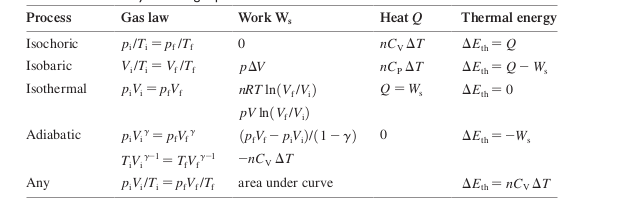
The Specific Heats of Gases

Isothermal

$$\mathrm{\Delta }{E}_{th}=0$$
$$W+Q=0$$

Isochoric

$$Q=n{C}_V\mathrm{\Delta }T$$
$$W=0,Q=\mathrm{\Delta }{E}_{th}$$

Isobaric

$$Q=n{C}_p\mathrm{\Delta }T$$

Any Ideal Process

• Any two processes that change the thermal energy by $\mathrm{\Delta }{E}_{th}$ will cause the same temperature change $\mathrm{\Delta }T$

• For any ideal-gas process
  $$\mathrm{\Delta }{E}_{th}=n{C}_v\mathrm{\Delta }T$$

• Heat depends on the path on the pV diagram

• Monatomic Gases: $$C_V=\frac{3}{2}R\approx 12.5$$

• Diatomic Gases: $$C_V=\frac{5}{2}\approx 20.8$$

• For all ideal gases: $$C_p-C_v=R$$

Adiabatic Process

$$W=n{C}_v\mathrm{\Delta }T$$
$$\gamma =\frac{C_P}{C_V}$$
$$p_f{V}_f^{\gamma }=p_i{V}_i^{\gamma }$$
$$T_f{V}_f^{\gamma -1}=T_i{V}_i^{\gamma -1}$$

• Image from wikipedia
  
• Temperature decreases during the adiabatic expansion
• Temperature increases during the adiabatic compression

Heat-Transfer Mechanisms

Conduction

$$\frac{dQ}{dt}=k\frac{A}{L}\mathrm{\Delta }T$$

• Thermal Conductivity: Represented by $k$
• $L$ denotes the thickness of the slab in between the two hot and cold regions and $A$ is the cross-sectional area
• Heat transferred through direct physical contact
• Heat flows due to a difference in temperature
• Conduction results do to the collision of particles at the interface between the two materials
  • Molecules from hotter region collide and transfer energy to those in an adjacent cooler region
• $k$ value is large for metals due to electrons

Convection

• Transfer of thermal energy by moving fluids
• Air is a poor conductor of heat, but thermal energy is transferred easily due to convection
• No simple equation due to turbulence

Radiation

• Electromagnetic waves carry energy
  $$\frac{dQ}{dt}=e\sigma A{T}^4$$
• Emissivity (e): How effectively a surface radiates energy
• Stefan-Boltzmann Constant ($\sigma$): $\sigma =5.67\cdot {10}^{-8}W/m^2{K}^4$
• Since objects emit and absorb radiation, the net amount of radiated power:
  $$\frac{d{Q}_{net}}{dt}=e\sigma A(T^4-T_0^4)$$
• Black body: Perfect absorber and emitter

20: The Micro/Macro Connection

Questions

We still have the following questions:

• Why does the ideal gas law work on every gas?
• Why is the molar specific heat ($C_v$) the same for all monatomic gases (12.5), diatomic gases (20.8), and elemental solids (25.0)?
• What is Temperature?
• Why does a gas have pressure?

Assumptions

• $N$ identical particles of mass $m$
• No intermolecular forces, so molecules only have kinetic energy, no potential energy
• Molecular motion is random (average speed is dependent on temperature)
• Collisions with the wall of the container are elastic

Molecular Speeds and Collisions

• There is a distribution of velocities for gas particles, not just one speed
• Pressure and temperature are based on the average of these speeds

Mean Free Path

• Mean Free Path ($\lambda$): The average distance between collisions
  • If a molecule has $N_{colli}$ collisions as it travels a distance $L$
    $$\lambda =\frac{L}{N_{colli}}$$
• Two molecules collide if the distance between their centers is less than $2r$
• The number of collisions is equal to the number of molecules in a cylindrical volume of length $L$ and radius of $2r$
  $$N_{colli}=\frac{N}{V}{V}_{cyl}=\frac{N}{V}\pi (2r{)}^{2}L=4\pi \frac{N}{V}{r}^{2}L$$
  $$\lambda =\frac{L}{N_{c}olli}=\frac{1}{4\pi (N/v)r^2}$$
• The above derivation assumed one particle was colliding with a stationary target particle. If we don’t assume this, we get the following:
  $$\lambda =\frac{1}{4\sqrt{2}\pi (N/v)r^2}$$

Pressure in a Gas

• Pressure comes from force over area. Force comes from change in momentum of a particle
  $$\mathrm{\Delta }{p}_x=-2m{v}_x$$
  $$\mathrm{\Delta }{P}_x=N_{colli}\mathrm{\Delta }{p}_x=-2N_{colli}m{v}_x$$

On average, half of the particles collide with the wall during the $\mathrm{\Delta }t$
$$N_{colli}=\frac{1}{2}n\mathrm{\Delta }V=\frac{1}{2}\frac{N}{V}A\mathrm{\Delta }L=\frac{1}{2}\frac{N}{V}A{v}_x\mathrm{\Delta }t$$
$$(F_{\text{on gas}}{)}_x=-\frac{2N_{colli}m{v}_x}{\mathrm{\Delta }t}$$
$$(F_{\text{on gas}}{)}_x=-(F_{\text{on wall}}{)}_x$$
$$F_{\text{on wall}}=\frac{N}{V}m(v_x^2{)}_{avg}A$$
$$p=\frac{mN}{V}\overline{v_x^2}$$

The Root-Mean-Square Speed

$$(v_x{)}_{avg}=0$$
$$v=(v_x^2+v_y^2+v_z^2{)}^{1/2}$$
$$(v^2{)}_{avg}=(v_x^2{)}_{avg}+(v_y^2{)}_{avg}+(v_z^2{)}_{avg}=3\overline{v_x^2}$$
$$v_{rms}=\sqrt{(v^2{)}_{avg}}$$
$$(v_x^2{)}_{avg}=(v_y^2{)}_{avg}=(v_z^2{)}_{avg}$$
$$(v_x^2{)}_{avg}=\frac{1}{3}{v}_{rms}^2$$
$$F_{\text{on wall}}=\frac{1}{3}\frac{N}{V}m{v}_{rms}^{2}A$$
$$p=\frac{1}{3}\frac{N}{V}m{v}_{rms}^2$$

Temperature

$${ϵ}_{avg}=\frac{1}{2}m(v^2{)}_{avg}=\frac{1}{2}m{v}_{rms}^2$$
$$p=\frac{2}{3}\frac{N}{V}{ϵ}_{avg}$$
$$pV=N{k}_{B}T$$
$${ϵ}_{avg}=\frac{3}{2}{k}_{B}T$$
Temperature is a measure of the average translational kinetic energy.

The following two equations relates macroscopic state variables ($T$ and $P$) to microscopic quantities:
$$p=\frac{2}{3}\frac{N}{V}{ϵ}_{avg}$$
$$T=\frac{2}{3k_B}{ϵ}_{avg}$$

We can assume collisions are elastic because if the collisions were inelastic, then the temperature of the gas would continue to decrease due to the loss of kinetic energy. This doesn’t happen in real life, so we can assume that collisions are elastic.

Thermal Energy and Specific Heat

$$E_{th}=K_{micro}+U_{micro}$$

Monatomic Gases

Atoms have no molecular bonds in an ideal gas so $U_{micro}=0$
$$E_{th}=K_{micro}=N{ϵ}_{avg}=\frac{3}{2}N{k}_{B}T=\frac{3}{2}nRT$$
$$\mathrm{\Delta }{E}_{th}=\frac{3}{2}nR\mathrm{\Delta }T$$
$$\mathrm{\Delta }{E}_{th}=n{C}_V\mathrm{\Delta }T$$
$$n{C}_V\mathrm{\Delta }T=\frac{3}{2}nR\mathrm{\Delta }T$$
$$C_v=\frac{3}{2}R=12.5J/(mol\cdot K)$$

Equipartition Theorem

• In addition to kinetic energy, non-monatomic gases can have the ofllowing forms of energy

1. Kinetic and potential energy associated with the vibrations from the spring like bond between molecules
2. Rotational Kinetic energy

• Degrees of Freedom: The number of independent modes of energy storage
  • Monatomic have 3 degrees of freedom since there are 3 different types of translational kinetic energy along x, y, and z
• Equipartition Theorem: The thermal energy is distributed evenly among all the different possible types of degrees of freedom. Each degree has the following energy: $\frac{1}{2}N{k}_{B}T$
  • Monatomic had 3 degrees so thermal energy was $\frac{3}{2}N{k}_{B}T$
• Vibration: For diatomic 2 degrees of freedom (one for each atom)
• Rotational: For diatomic only 2 degrees (since rotation along one axis has no rotational kinetic energy)

Solids

• 6 degrees of freedom
  • 3 translational kinetic and 3 vibrational (potential)
    $$E_{th}=3N{k}_{B}T=3nRT$$

Diatomic Molecules

• 8 total degrees of freedom but only 5 are available at room temperature due to quantum effects
  $$E_{th}=\frac{5}{2}N{k}_{B}T=\frac{5}{2}nRT$$
  $$C_v=\frac{5}{2}R$$
  $C_v$ is $\frac{3}{2}R$ at very low temperatures and $\frac{7}{2}R$ at high temperatures

Thermal Interactions and Heat

• Heat is the energy transferred via collisions
• When thermal equilibrium is reached the following is true
  $$({ϵ}_1{)}_{avg}=({ϵ}_2{)}_{avg}$$
  $$T_{1f}=T_{2f}$$

Second Law of Thermodynamics

• Equilibrium is the most probable state

• Entropy: Measures the probability that a macroscopic state will occur spontaneously or the measure of disorder

• Reversible microscopic events lead to irreversible macroscopic behavior since some macroscopic states are more probable

• Second Law of Thermodynamics: The entropy of a system never decreases

  • Heat always travels from hot to cold

21: Heat Engines and Refrigerators

• Practical devices transform heat into work
• All devices must obey two two laws of thermodynamics
  1. Energy is conserved $$\mathrm{\Delta }{E}_{th}=W_{\text{done on system}}+Q$$
  2. Most macroscopic processes are irreversible. Heat energy is transferred spontaneously from a hooter system to a cold system but never the other way around

Questions

1. What are the limitations imposed by the above laws on these practical devices
2. How do these devices transform heat into work?

Heat into Work

• So far we’ve defined $W$ as the work done on the system (by an external force). Now we define $W_s$ as the work done by the system, since we only care about that when talking about practical devices.
  $$\mathrm{\Delta }{E}_{th}=W+Q$$
  $$W=-W_s$$
  $$\mathrm{\Delta }{E}_{th}=-W_s+Q$$
  $$Q=\mathrm{\Delta }{E}_{th}+W_s$$

• Energy is transferred into the system as heat to do work or stored within the system as increased thermal energy

• Heat Reservoir: An object that is so large that its temperature does not change when heat is transferred between the system and reservoir

• $Q_H$: Amount of heat transferred into a hot reservoir called

• $Q_C$: Amount of heat transferred into a cold reservoir

• By definition $Q_C$ and $Q_H$ are always positive since they only show magnitude

• Converting heat to work can be done with thermal expansion, but the system is at a different state. A heat engine must be a closed cycle.

Heat Engine

• Clockwise PV diagram

1. Extract heat, $H_S$ from hot reservoir
2. Do useful work
3. Exhausts heat energy ($Q_c$) to colder reservoir

Sterling Engine

• Two isotherms and two isochoric processes in one cycle
• Heat transfers occur in all four processes

Thermal Efficiency

• The purpose of heat engines is to transform as much of the heat absorbed $Q_H$ into work done $W_{out}$
• Thermal Efficiency is denoted by $\eta$
  $$\eta =\frac{W_{out}}{Q_H}$$

$$W_{out}=Q_{net}=Q_H-Q_C$$
$$\eta =1-\frac{Q_C}{Q_H}$$

• Actual engines have $\eta$ of 0.1 to 0.5

Ideal-Gas Heat Engines

• An ideal gas heat engine can be represented by a clock-wise loop
• The net work is the area inside the loop, not the area under the loop

Refrigerator

Opposite of heat engine (Counter clockwise PV diagram)

• $W_{in}$ and $Q_c$ as inputs
  • $W_{in}$ is the work done on the system
• $Q_H$ as output
• A Refrigerator transfers heat out of its cooler interior to its warmer surroundings
• Refrigerators don’t violate the 2nd Law since you have to “pay” to have heat flow from $T_c$ to $T_H$
  • Requires $W_{in}$ (work input)
• In any closed-cycle refrigerator, all state variables return to their initial values once every cycle
• Over one cycle: $\mathrm{\Delta }{E}_{th}=0$
• 1st Law
  $$Q_H=Q_C+W_{in}$$

Efficiency

$$K=\frac{Q_c}{W_{in}}=\frac{\text{what you get}}{\text{what you had to pay}}$$
$K$ tends to infinity for a perfect refrigerator since $W_{i}n$ decreases as efficiency increases.

Brayton Cycle

• Ideal-Gas refrigerator that uses adiabatic compression and adiabatic expansion to quickly heat and cool system, respectively

1. Two adiabatic processes
2. Two isobaric processes

• Reverse Brayton cycle is for refrigerators and regular is for heat engines

No Perfect Heat Engine

• No perfect heat engine with $\eta =1$
• A Perfect Heat Engine means $Q_c=0$. We could use its work output as the work input to an ordinary refrigerator. Leads to spontaneous transfer from $Q_{C}to{Q}_H$.
• This combo violates the second law. Thus all heat engines MUST output some $Q_c$

Limits of Efficiency

• Question: Is there a maximum efficiency or max COP (Coefficient of performance) for a device operating between $T_C$ and $T_H$

• Answer: Yes

Carnot Engine

• Carnot Engine: Perfectly reversible engine
• Carnot Cycle
  1. Two Adiabatic processes ($Q=0$)
  2. Two isothermal processes ($\mathrm{\Delta }{E}_{th}=0$)
     $$\frac{Q_C}{Q_H}=\frac{T_C}{T_H}$$
     $${\eta }_{carnot}=1-\frac{T_C}{T_H}$$

Maximum Efficiency

• Second Law (informal statement): No heat engine operating between energy reservoirs at $T_H$ and $T_C$ can exceed the Carnot efficiency
  $$\eta =\frac{W_{out}}{Q_H}\le {\eta }_{carnot}=1-\frac{T_C}{T_H}$$
• Second Law (informal statement): No refrigerator operating between energy reservoirs at $T_H$ and $T_C$ can exceed the Carnot COP

22: Electric Charge and Force

• Goal: Learn to calculate and use the electric field
• Questions

1. What is Coulomb’s Law?
2. How to determine the electric force on a point charge?
3. What is an electric field?
4. What is the electric fields of a point charge?
5. How to calculate the electric field of discrete charge distribution?

Electric Charges

• Proton and electron

Electric Forces

• Coulomb’s Law: A force occurs for point charges that are separated by a distance $r$
• For two positively/negatively charged particles, they experience a repulsive force of the magnitude.
  $$F_{\text{1 on 2}}=F_{\text{2 on 1}}=\frac{K|q_1||q_2|}{r^2}$$
• $K$ is the electrostatic constant
  $$K=8.99\times {10}^{9}N\cdot m^2/C^2=\frac{1}{4\pi {ϵ}_0}$$
• Permittivity constant ${ϵ}_0$
• Charge of one electron or proton is $1.6\times {10}^{-19}C$
  $$F=\frac{1}{4\pi {ϵ}_0}\frac{|q_1||q_2|}{r^2}$$

Forces on Point Charges

• Add up vectors
  Use coulomb’s Law to get magnitudes

The Field Model

23: The Electric Field

• Electric field created by charge

• The Electric Model

• Long range of interaction a distance
  $$\overrightarrow{E}(x,y,z)=\frac{\overrightarrow{F}\text{ at }(x,y,z)}{q}$$

• Unit of Electric field are $\frac{N}{C}$ and the magnitude is the electric field strength

• In the Field Diagram for protons, the field lines points a away from from source. For an electron, the source acts as a sink.
  $$\overrightarrow{E}=\frac{1}{4\pi {ϵ}_0}\frac{q}{r^2}\hat{r}$$
  $r$ is from the source charge to the test charge

The Dipole: An Important Charge Distribution

• Electric dipole: Consists of two point charges of equal magnitude but opposite signs, held a short distance apart
• Many molecules can be modeled as dipoles (e.g. water)

For a point lying on the axis of the dipole
$$E=\frac{1}{4\pi {ϵ}_0}\frac{2qd}{r^3}$$

For a point perpendicular to the dipole
$$E=-\frac{1}{4\pi {ϵ}_0}\frac{qd}{r^3}$$

Where $d$ is the distance between the dipoles

$r$ is the distance from the center of the dipole. Above only works if $r»d$

Continuous Charge Distributions

Question: What if the charge is continuous (not discrete)?

For macroscopic charged objects, like rods or disks, we assume the charge has a continuous distribution.

1. Divide the objects into small point charge-like pieces $dq$. Each piece creates a small $dE$
2. The summation of fields of an infinite number of infinitesimally small pieces means integration.

$$\overrightarrow{E}(P)=\int d\overrightarrow{E}=\int \frac{kdq}{r^2}\hat{r}$$

An Infinite Line of Charge

• A straight infinite line of charge coincides with the x-axis and the line carries uniform charge with the charge density $\lambda$ (C/m).
• The x-component of two equidistant points on the line will cancel out
• Only the y-component adds up
  $$d{E}_y=dE\cos \theta$$
  $$dE=k\lambda \frac{dx}{r^2},\cos \theta =\frac{y}{r}$$
  $$d{E}_y=k\lambda \frac{dx}{r^3}$$
  with $r=\sqrt{(x^2+y^2)}$

$$E=E_y={\int }_{-\mathrm{\infty }}^{\mathrm{\infty }}\frac{k\lambda ydx}{(x^2+y^2{)}^{\frac{3}{2}}}=k\lambda y{\int }_{-\mathrm{\infty }}^{\mathrm{\infty }}\frac{dx}{(x^2+y^2{)}^{\frac{3}{2}}}$$
$$\overrightarrow{E}(P)=\frac{2k\lambda }{y}\hat{j}$$

• Notice that the electric field is proportional to $\frac{1}{distance}$ instead of $\frac{1}{distanc{e}^2}$ like for a point charge

Ring of Charge

• A ring of radius $a$ carries a charge $Q$ distributed evenly over the ring. At any point $P$ on the x-axis, there is $dE$ and $dq$, where the x-axis passes through the center of the ring
  $$r=\sqrt{x^2+a^2}$$
• Only x-components add up

$$E={\int }_{ring}d{E}_x={\int }_{ring}\frac{kxdq}{{\sqrt{x^2+a^2}}^3}=\frac{kx}{{\sqrt{x^2+a^2}}^3}{\int }_{ring}dq$$
$$\overrightarrow{E}\left(P\right)=\frac{kQx}{(x^2+a^2{)}^{\frac{3}{2}}}\hat{i}$$

• At the center of the ring, the net electric field is 0

Disk of Charge

$$\eta =\frac{Q}{A}=\text{charge density}$$
$$E_{disk}=\frac{\eta }{2{ϵ}_0}(1-\frac{z}{\sqrt{z^2+R^2}})$$

where the z-axis passes through the center of the disk and the point lies on the z-axis

Infinite Plane of Charge

• An infinite plane is just a disk with radius of infinity
  $$E_{plane}=\frac{\eta }{2{ϵ}_0}$$

• The electric field is the same at any point in space regardless of how “far” away a point is from the plane, since the plane is infinite

• $E$ is away from the plane if the charge is + and towards the plane if charge is -

Sphere of Charge

$${\overrightarrow{E}}_{sphere}=\frac{Q}{4\pi {ϵ}_0{r}^2}\hat{r},r\ge R$$

Parallel-Plate Capacitor

• One plane is positively charged and one plane is negatively charged
• All charges are on one surface of hte plane because opposite charges attract
• $E=0$ outside the capacitor
• For inside the capacitor
  $$E=\frac{Q}{{ϵ}_{0}A}$$
• A uniform electric field exists inside a parallel-plate capacitor

25: The Electric Potential

Potential from the Electric Field

• Like gravity, the force exerted on a charge $q$, by the electric field is conservative

• Work can be represented by the change of electric potential energy
  $$\mathrm{\Delta }U=U(B)-U(A)$$
  $$\mathrm{\Delta }U=-W(A\to B)=-{\int }_A^B\overrightarrow{F}\cdot d\overrightarrow{r}$$

• $r$ is the positive vector along any path from point $A$ to point $B$

• Potential Difference:
  $$\mathrm{\Delta }{V}_{AB}=\frac{\mathrm{\Delta }{U}_{AB}}{q}=-{\int }_A^B\overrightarrow{E}\cdot d\overrightarrow{r}$$

  • Must define a reference point (V(A) = 0)

Potential Difference :Capacitor

A plate is equipotent

• Define reference point $A$ to be $0$
  $$V_B=-{\int }_A^B\overrightarrow{E}\cdot d\overrightarrow{r}$$

• Choose path as straight line
  $$E=-E\hat{i}$$
  $$d\overrightarrow{r}=dx\hat{i}$$
  $$d\overrightarrow{r}=dy\hat{i}$$

• Notice that since $E$ is only in the $x$ direction, the contribution from the $y$ is $0$
  $$V_B=-{\int }_A^B\overrightarrow{E}\cdot d\overrightarrow{r}={\int }_0^{X}Edx=Ex$$
  Insert Diagram

• The electric potential decreases in the direction of the electric field

• When U increases, K decreases, and vice versa

• Positive charge: “downhill” means U goes down and K goes up

Electric Potential of a Point Charge

Insert Diagram

• Easier to use a path parallel to $r_A$ and $r_B$

$$\mathrm{\Delta }{V}_{AB}=\frac{\mathrm{\Delta }{U}_{AB}}{q}$$

$$\overrightarrow{E}=\frac{kq}{r^2}\overrightarrow{r}$$
$$d\overrightarrow{dr}=dr\overrightarrow{r}$$

$$\mathrm{\Delta }{V}_{ab}=-{\int }_{r_A}^{r_B}\frac{kq}{r^2}dr=-kq{\int }_{R_A}^{R_B}\frac{dr}{r^2}=kq(\frac{1}{r_B}-\frac{1}{r_A})$$

• Notice that the second part of the path (the curve) is always perpendicular to the electric field. This means the contribution is $0$ to the electric field along that $r$.

$$V_{\text{point charge}}=\frac{1}{4\pi {ϵ}_0}\frac{q}{r}$$

Electric Potential of a Charged Sphere

• Using Gauss’s Law, we know that outside the sphere, the field is the same as a point charge
  $$V=\frac{1}{4\pi {ϵ}_0}\frac{Q}{r},r\ge R$$

If the potential at the surface $V_0$ is known, the potential at $r$ is
$$V=\frac{R}{r}{V}_0$$

Electric Potential for Multiple Charges

• You can add electric potentials

Electric Potential for Ring

% $$V(P)=\int dV=\int \frac{kdq}{r}$$

26: Potential and Field

Capacitors

$$C_{parallel}=C_1+C_2+C_3\dots$$
$$\frac{1}{C_{serial}}=\frac{1}{C_1}+\frac{1}{C_2}+\frac{1}{C_3}+\dots$$

$$Q=C\mathrm{\Delta }V$$

• If two capacitors $C_1$ and $C_2$ are in series, then $Q_{12}=Q_1=Q_2$
• The potential difference across two capacitors, $C_1$ and $C_2$ in parallel is the same
  $$V_{12}=V_1=V_2$$

Capacitance in Terms of Distance and Area

For a parallel-plate capacitor
$$C=\frac{{ϵ}_{0}A}{d}=\frac{Q}{\mathrm{\Delta }{V}_C}$$

27: Current and Resistance

Current

• Weakly bound valence in metals
• Normally electrons are moving randomly with no net flow of charge
• An electric field causes a slow drift at speed $v_d$
  $$i_e=n_{e}A{v}_d$$

$v_d$ is the drift speed of the electrons (net motion of electrons “flowing”)

• Very small value
  $n_e$ is the number density (electrons in a given volume)

• $A$ is cross sectional area

• $i_e$ is the number of electrons flowing per time through a certain area

• Most metals contribute 1 valence electron to the sea of electrons per atom

• The number of electrons $n_e$ (number of electrons per cubic meter) is the same as the number of atoms per cubic meter

Creating a Current

• $\overrightarrow{E}=0$ inside a conductor in static equilibrium
• When charges are moving, there is a non-zero electric field causing electrons to move and current to flow

$$i_e=\frac{n_{e}e\tau A}{m}E$$

• $\tau$ is the mean time between collision (property of the conductor)

$$I=\frac{Q}{\mathrm{\Delta }t}=\frac{e{N}_e}{\mathrm{\Delta }t}=e{i}_e$$
$I$ is the charge per time

Current is defined as the direction positive charges flow, so current is opposite the direction electrons flow

Conservation of Current and the Junction Rule

Law 1

Due to conservation of charge, the current must be the same at all cross-sections along a current-carrying wire

Law 2 (Kirchhoff’s Junction Law)

For a junction, the law of conservation of current requires that the sum of the current in the branches

$$\sum I_{in}=\sum I_{out}$$

Conductivity and Resistivity

$$v_x=v_{0x}+a\mathrm{\Delta }t=v_{0x}+\left(\frac{eE}{m}\right)\mathrm{\Delta }t$$

• Assume $v_{0x}=0$ and $\tau =\mathrm{\Delta }t$ for all collisions
  $$v_d=\frac{e\tau }{m}E$$
• Average Time between Collisions/Electron Lifetime/Scattering Time: $\tau$ is a material dependent quantity
  $$J=\frac{dI}{dA}=n_{e}e{v}_d=\frac{n_e{e}^2\tau }{m}E$$
  $J$ is the current density and $\frac{n_e{e}^2\tau }{m}$ only depends on the conducting material
  $$\sigma =\text{conductivity}=\frac{n_e{e}^2\tau }{m}$$
  $$J=\sigma E$$

1. Current is caused by an electric field
2. Current density depends on the strength of the electric field
3. Current density depends on the material’s conductivity

When $J(p)$ varies point to points, the current through an area is the surface integral of the current density over that area
$$dI=JdA$$
$$I={\int }_{area}\overrightarrow{J}\cdot d\overrightarrow{A}$$

$$\rho =\text{resistivity}=\frac{1}{\sigma }$$

$$R=\text{resistance}=\frac{\rho L}{A}$$

Superconductivity

• Resistance is actually zero
• Charge moves without an electric field

Ohm’s Law

If we assume the electric field is uniform:
$$\mathrm{\Delta }V=E\cdot L$$
Remember $E=\frac{F}{q}=\frac{\mathrm{\Delta }V}{d}$

$$E_s=-dV/ds⟹E=\frac{\mathrm{\Delta }V}{\mathrm{\Delta }s}$$
If we assume $J$ is uniform and perpendicular to the cross section
$$I=JA=A\sigma E=\frac{A}{\rho }E=\frac{A}{\rho L}\mathrm{\Delta }V$$
$$I=\frac{\mathrm{\Delta }V}{R}$$

28: Fundamentals of Circuits

Kirchoff’s Loop Law

For a loop (any path that starts and ends at the same point), the law of conservation of energy requires
$$\mathrm{\Delta }{V}_{loop}=\sum (\mathrm{\Delta }V{)}_i=0$$

Note: this can be true only if at least one $(\mathrm{\Delta }V{)}_i$ is positive (there is a power supply).

Let us define $\mathrm{\Delta }V$ to be negative for resistors and any component that consumes electricity.

• From negative to positive for a battery: $\mathrm{\Delta }V=+ϵ$
• From positive to negative for a battery: $\mathrm{\Delta }V=-ϵ$
• From positive to negative for a resistor: $\mathrm{\Delta }V=-\mathrm{\Delta }{V}_R=-IR$

Energy and Power

The rate of transfer of thermal energy through a resistor
$$P_R=\frac{d{E}_{th}}{dt}=\frac{dq}{dt}\mathrm{\Delta }{V}_R=I\mathrm{\Delta }{V}_R=I^{2}R=\frac{(\mathrm{\Delta }V{)}^2}{R}$$

29: Magnetism

• Magnetic fields are similar to electric field, except that magnetic fields can only exist as dipoles

• The force on a north pole is parallel to $\overrightarrow{B}$ while the force on a south pole is opposite to $\overrightarrow{B}$.

Magnetic Field of a Moving Charge

• Biot-Savart Law
  $${\overrightarrow{B}}_{\text{point charge}}=\frac{{\mu }_0}{4\pi }\frac{q\overrightarrow{v}\times \hat{r}}{r^2}$$
• The above is analogous to Coulomb’s Law

Superposition of Magnetic Fields

$${\overrightarrow{B}}_{tota}=\overrightarrow{B_1}+\overrightarrow{B_2}+\dots +{\overrightarrow{B}}_n$$
Add magnetic fields vectorally, the $\hat{r}$ unit vector will be different for each of the individual magnetic fields

Magnetic Field of a Long Straight Wire

$$\mathrm{\Delta }Q\overrightarrow{v}=I\mathrm{\Delta }\overrightarrow{s}$$
$$d\overrightarrow{B}=\frac{{\mu }_0}{4\pi }\frac{I\mathrm{\Delta }\overrightarrow{s}\times \hat{r}}{r^2}$$
where $s$ is the length of the wire

Infinite Wire

$$B_{wire}=\int d\overrightarrow{B}=\frac{{\mu }_{0}I}{2\pi r}$$

N -Turn Current Loop

$$B_{\text{coil center}}=\frac{{\mu }_{0}NI}{2R}$$

Magnetic Field of a Current Loop

On axis magnetic field (axis through center of loop):
$$\overrightarrow{B}(P)=\frac{{\mu }_{0}I{a}^2}{2(x^2+a^2{)}^{3/2}}\hat{i}$$

For large distances $|x|»a$ the following is true
$$B=\frac{{\mu }_{0}I{a}^2}{2|x{|}^3}=\frac{{\mu }_{0}IA}{2\pi |x{|}^3}$$

Solenoid

$$n=N/L$$
$$B={\mu }_{0}nI={\mu }_0\frac{N}{L}I$$

Magnetic Dipole Moment

A current loop is a magnetic dipole.
$$\overrightarrow{\mu }=\text{Magnetic Dipole Moment}=NIA$$

Magnetic Dipole is always perpendicular to the area of the loop (from south to north pole)

$${\overrightarrow{B}}_{dipole}=\frac{{\mu }_{0}2\overrightarrow{\mu }}{4\pi |x^3|}$$
direction above is on the axis of the magnetic dipole

Cyclotron

$$F=qvB=\frac{m{v}^2}{r}$$
$$r=\frac{mv}{qB}$$

Cyclotron frequency (1/T)
$$f=\frac{1}{T}=\frac{v}{2\pi r}=\frac{v}{2\pi (mv/qB)}=\frac{qB}{2\pi m}$$

Cyclotron frequency does not depend on the speed of the particle!!!!

When the particle has a component of $\mathbf{v}$ along the field $B$, it forms a helix/spiral

• Perpendicular component is responsible for circular motion
• The parallel component is responsible for

Spectrometer: Charged Particle in B

1. Positive ions of charge $q$ and $m$ are accelerated from rest by a potential difference $\mathrm{\Delta }V$

$$\frac{1}{2}m{v}^2=q\mathrm{\Delta }V$$

2. The particles follow a Clockwise (If $q>0$) circular path in uniform magnetic field (out of screen). After half an orbit, they land on detector

Find $d$ (diameter)

$$d=2r=\frac{2mv}{qB}=\frac{2m}{qB}\sqrt{\frac{2q\mathrm{\Delta }V}{m}}=2\sqrt{\frac{2m\mathrm{\Delta }V}{q{B}^2}}$$

Magnetic Force on a Current

$$\overrightarrow{F}=q\overrightarrow{v}\times \overrightarrow{B}$$
Consider a segment of length $L$ in which the charges $Q$ have a drift velocity of $v_d$

$$\overrightarrow{F_q}=q\overrightarrow{v_d}\times \overrightarrow{B}$$
$$Q{v}_d=IL⟹$$

$$\overrightarrow{F}=I\overrightarrow{L}\times \overrightarrow{B}$$

Note: $I$ is always in direction of $\overrightarrow{L}$

Magnetic Force Between Parallel Wires

If two parallel wires have currents that both go up, they will attract.

The wire on the left creates a magnetic field that goes into the page on the right wire. So the right wire is pulled to the left. The right wire creates a magnetic field out of the page on the left wire. Thus the left wire has a force to the right.

$$F_{\text{parallel wires}}=\frac{{\mu }_{0}l{I}_1{I}_2}{2\pi d}$$

Forces and Torques on Loops

We know a current loop is a magnetic dipole
Consider a $l\times l$ current loop with current $I$ in uniform $B$ making angle $\theta$ with the field

$$d=\frac{1}{2}l\sin \theta$$
$$\tau =2Fd=2IlB\frac{1}{2}l\sin \theta =I{l}^{2}B\sin \theta =IAB\sin \theta =\mu B\sin \theta$$

$$\overrightarrow{\tau }=\overrightarrow{\mu }\times \overrightarrow{B}$$

Applicable to any loop of any shape

30: Electromagnetic Induction

Induced Current

Question: If electric currents produce magnetic fields, is the reverse possible?

Magnetic Flux

$$\text{Number of lines through an area dA}=\overrightarrow{B}\cdot d\overrightarrow{A}$$

Magnetic flux of $\overrightarrow{B}$ through a loop, denoted by $\mathrm{\Phi }$, counts the total number of lines passing through that loop

$${\mathrm{\Phi }}_m=\int \overrightarrow{B}\cdot d\overrightarrow{A}$$

Note that the $\overrightarrow{A}$ vector is the normal vector through the loop

• $\theta$ is the angle between $\overrightarrow{B}$ and the normal vector $\overrightarrow{A}$

$${\mathrm{\Phi }}_m=AB\cos \theta$$

When $\theta =0$, the magnetic field is parallel to the normal vector of the loop. In other words, the magnetic field is perpendicular to the loop’s area.

1 weber = 1 Wb = 1 $T\cdot m^2$

Faraday’s Law

$$\epsilon =\left|\frac{d{\varphi }_M}{dt}\right|=|\frac{d}{dt}(AB\cos \theta )|=|A\frac{d}{dt}(B\cos \theta )+B\frac{d}{dt}(A\cos \theta )|$$

If we slide a conducting wire along a U-shaped conducting rail:
$$\epsilon =\frac{d}{dt}(xlB)=\frac{dx}{dt}lB=vlB$$

$$I=\frac{\epsilon }{R}=\frac{vlB}{R}$$

Lenz’s Law

• Question: Which direction is the induced current
• An induced current always moves in the direction that its magnetic field opposes the original change of flux
  The magnetic field ${\overrightarrow{B}}_{induced}$ due to the induced current points

1. in the opposite direction to the original $\overrightarrow{B}$ if the flux is increasing
2. in the same direction as the original $\overrightarrow{B}$ if the flux is decreasing
3. is zero if the flux is not changing

Induced Electric Fields

• There must be an induced electric field tangent to the loop at all points
• EMF = the work per unit charge done as a charge goes around a closed loop
  $$\epsilon =\left|\frac{d\varphi }{dt}\right|=A\left|\frac{dB}{dt}\right|$$
  $$W=q\oint \overrightarrow{E}\cdot d\overrightarrow{s}$$
  $$\epsilon =\frac{W}{q}$$
  $$⟹\oint \overrightarrow{E}\cdot d\overrightarrow{s}=\left|\frac{d\varphi }{dt}\right|$$
  For an induced electric field that is produced by a changing magnetic field producing “pinwheel” pattern of induced electric fields
  $$\oint \overrightarrow{E}\cdot d\overrightarrow{s}=2\pi rE=\left|\frac{d\varphi }{dt}\right|$$
  where $r$ is the distance from the center
  And the area of the magnetic flux is only the area formed by the real or imaginary closed curve of integration (loop)

Solenoid Induced Electric Field

$$E_{inside}=\frac{r}{2}\left|\frac{\mathrm{d}B}{\mathrm{d}t}\right|$$

Generalization of Faraday’s Law

$$\oint \overrightarrow{E}\cdot d\overrightarrow{s}=-\frac{d\varphi }{dt}$$

• Direction of electric field follows Lenz’s Law

Mutual Inductance

Suppose there are two coils: Coil 1 has a changing current $I_1$ and generates a changing magnetic field. Coil 2 is close to coil 1 and has an induced EMF from Coil 1.

Inductance is a property of Coil 2, denoted by $M_{21}$, measured in Henry ($\frac{T\cdot m^2}{A}$)
$$M_{21}=\frac{{\varphi }_2}{I_1}$$
$${\epsilon }_2=-M_{21}\frac{d{I}_1}{dt}$$

Self-Inductance

A changing current in a coil wil also induce an EMF ${\epsilon }_L$ in itself
$${\epsilon }_L=-L\frac{dI}{dt}$$

$L$ is the self inductance
$$L=\frac{\varphi }{I}$$

Example: For solenoid of length $l$
$$L=\frac{\varphi }{I}=\frac{NBA}{I}=\frac{{\mu }_0{N}^{2}A}{l}={\mu }_0{n}^{2}Al$$

Magnetic Energy in an Inductor

• Energy can be stored in an electric field of a capacitor
• Similarly, energy can be stored in a magnetic field of an inductor
  $$U=L{\int }_0^{I}IdI=\frac{1}{2}L{I}^2$$

Magnetic Energy Density

• For an ideal solenoid
  $$L={\mu }_0{n}^{2}Al$$
  $$B={\mu }_{0}nI$$

$$U=\frac{1}{2}L{I}^2=\frac{1}{2}\frac{B^2}{{\mu }_0}Al$$

Energy per unit volume, Magnetic Energy Density
$$u_B=\frac{B^2}{2{\mu }_0}$$

Although the energy density was derived via a solenoid, these equations are universal.

Generators

$${\varphi }_m=\overrightarrow{A}\cdot \overrightarrow{b}=AB\cos \theta =AB\cos \omega t$$
$$\omega =2\pi f$$
$${\epsilon }_{coil}=-N\frac{\mathrm{d}{\varphi }_m}{\mathrm{d}t}=-ABN\frac{\mathrm{d}}{\mathrm{d}t}(\cos \omega t)=\omega ABN\sin \omega t$$

Transformers

$S$ = Secondary
$P$ = Primary
$$\frac{N_S}{N_P}=\frac{V_S}{V_P}$$

31: Electromagnetic Fields and Waves

Maxwell’s Law

1. $\oint \overrightarrow{E}\cdot d\overrightarrow{A}=\frac{Q_{i}n}{{ϵ}_0}$

• Charged particles create an electric field

2. $\oint \overrightarrow{B}\cdot d\overrightarrow{A}=0$

• There are no isolated magnetic poles

3. $\oint \overrightarrow{E}\cdot d\overrightarrow{s}=-\frac{d{\varphi }_m}{dt}$

• An electric field can also be created by a changing magnetic field

4. $\oint \overrightarrow{B}\cdot d\overrightarrow{s}={\mu }_0{I}_{through}+{ϵ}_0{\mu }_0\frac{d{\varphi }_e}{dt}$

• Currents (or changing electric flux) create a magnetic field

Maxwell’s Correction to Ampere’s Law

• Ampere’s Law only works for steady currents

• An example of when ampere’s law fails is with a capacitor

• A changing electric field flux can also create magnetic field as well

  • ${\varphi }_e$ increases as the capacitor charges

• The electric field is $$E=\frac{Q}{{ϵ}_{0}A}$$

• The electric flux (through $S_2$) is $${\varphi }_e=E\ast A=\frac{Q}{{ϵ}_0}$$

• The rate the flux changes (through $S_2$ assuming $A$ doesn’t change)
  $$\frac{d{\varphi }_e}{dt}=\frac{1}{{ϵ}_0}\frac{dQ}{dt}=\frac{I}{{ϵ}_0}$$

• Maxwell added a correction term to Ampere’s Law called the displacement current
  $$I_{disp}={ϵ}_0\frac{d{\varphi }_e}{dt}$$

Ampere-Maxwell (AM) Law

• The A-M law states that either a changing electric flux or electric current through a closed loop creates a magnetic flux around the loop
• A magnetic field can be created either by an electric current or by a changing electric field
  $$\oint \overrightarrow{B}\cdot d\overrightarrow{s}={\mu }_0(I_{through}+I_{dist})={\mu }_0(I_{through}+{ϵ}_0\frac{d{\varphi }_e}{dt})$$

Maxwell’s Equations in Vacuum (Special Case)

• In a vacuum (empty space) there is no electric charge ($q=0$) and no current ($I=0$) since there is no wire

Gauss’s Law ($\overrightarrow{E}$)
$$\oint \overrightarrow{E}\cdot d\overrightarrow{A}=0$$
Gauss’s Law ($\overrightarrow{B}$)
$$\oint \overrightarrow{E}\cdot d\overrightarrow{r}=-\frac{d{\varphi }_B}{dt}$$
Faraday
$$\oint \overrightarrow{B}\cdot d\overrightarrow{A}=0$$
Ampere
$$\oint \overrightarrow{B}\cdot d\overrightarrow{r}={\mu }_0{ϵ}_0\frac{d{\varphi }_E}{dt}$$

• Complete symmetry between magnetic field and electric field
• The only source of either field is the change in time of the other field

Plane Waves

• Simplest solution of Maxwell’s equations is the plane wave
• A plane wave consists of E&M fields that vary in space ONLY in the direction of the wave propagation
• The plane is normal to the direction of propagation
• The electric field and magnetic field is the same everywhere on the plane

$$E_y=E_0\sin (kx-\omega t)$$
$$B_z=B_0\sin (kx-\omega t)$$
Let the $E$ be only along the $y$ axis and $B$ along the z-axis and let the wave move in the direction of the x-axis
$\overrightarrow{E}\times \overrightarrow{B}$ is the direction of the propagation (x-axis)

Properties of Plane EM Waves

• Wave Number: $k=\frac{2\pi }{\lambda }$ Describes variation of wave with respect to $x$

• Angular Frequency: $\omega =2\pi f=\frac{2\pi }{T}$ Variation of wave with respect to $t$

• Velocity $v=\lambda f=\frac{\omega }{k}$

• The plane wave only satisfies Maxwell’s equations in a vacuum if the wave speed is given by
  $$v=\frac{\omega }{k}=\frac{1}{\sqrt{{ϵ}_0{\mu }_0}}=c=3.0\cdot {10}^{8}m/s$$

Results

1. Light is an EM wave
2. Optics can be viewed as a branch of E&M

$$E=\frac{\omega }{k}B=cB$$

Intensity and Power

$$\overrightarrow{S}=\frac{1}{{\mu }_0}\overrightarrow{E}\times \overrightarrow{B}$$
The Poynting vector, $\overrightarrow{S}$ points in the direction the EM wave is traveling.

$$I=\frac{P}{A}=S_{avg}=\frac{1}{2c{\mu }_0}{E}_0^2=\frac{c{ϵ}_0}{2}{E}_0^2$$
The above relates the intensity of an EM wave to the amplitude of the wave’s electric field

$$I=\frac{P_{source}}{4\pi r^2}$$

Radiation Pressure

$$F=\frac{\mathrm{\Delta }p}{\mathrm{\Delta }t}=\frac{P}{c}$$
where $P$ is power and $p$ momentum

$$p_{rad}=\frac{F}{A}=\frac{P/A}{c}=\frac{I}{c}$$
where $p_{rad}$ is radiation pressure

Polarization

Electric field vector and Poynting vector define the plane of polarization

Malus’s Law

$$I=I_0{\cos }^2\theta$$

33: Ray Optics

Ray Model of Light

• Light travels in straight lines
• Rays can cross without disturbing each other
• Rays travel forever until they interact with matter
• Objects are sources of light rays

Law of Reflection

• The incident ray and reflected ray are in the same plane normal to the surface
• The angle of reflection equals the angle of incidence
  $${\theta }_i={\theta }_f$$

Refraction

Snell’s Law

$$n_1\sin {\theta }_1=n_2\sin {\theta }_2$$

• If $n_2>n_1$, then $\theta 2<{\theta }_1$, then light bends towards the normal
• Bending occurs because the wavelength $\lambda$ decreases in more dense media since $v$ also decreases $v=f\lambda$

$$v_{medium}=\frac{c}{n}$$

Mirrors

• Flat: Virtual image only
  $$s^{\prime }=s$$

• Parabolic: All rays parallel to mirror axis converge to single focal point

• Spherical Mirror: Approximates parabolic mirror close to the mirror
  $$f=r/2$$

• Focal Point (F): Any incoming parallel rays will be reflected towards this focal point

• Center Point (C): The distance from this point to the mirror is the same in any direction

• Real Image: Where two (or more) light rays converge

• Virtual Image: An image formed when diverging rays appear to meet at a point “behind” the mirror

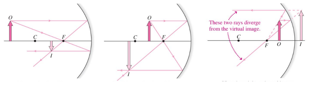
Concave Mirror

• Concave mirrors can create either real or virtual mirrors
  • If $s>2f$, the image is real, inverted, and reduced in size
  • If $2f>s>f$, the image is real, inverted, and enlarged
  • If $s<f$, the image is virtual, upright, and enlarged
    • Note that for a flat mirror, this is the case. The reflection is virtual and the focal pint is infinitely away from the mirror

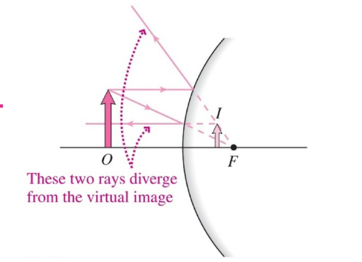
Convex Mirror

• Incoming rays reflects on the outside of its spherical curvature, causing light to diverge
• Features

1. The focal point is behind the mirror ($f<0$)
2. The image is virtual, upright, and reduced in size

Mirror and Magnification equations

• If the image, focal point, or center of curvature is on the reflecting side of the mirror, the corresponding distance ($s^{\prime }$, $f$, $R$) is positive and negative otherwise

$$M=\frac{h^{\prime }}{h}=\frac{-s^{\prime }}{s}$$

• $M$ is magnification
• $h^{\prime }$ is the new height of the image and $h$ is the height of the original image
• $s^{\prime }$ and $s$ correspond to the distance from the mirror for the new and old images, respectively

$$\frac{1}{s}+\frac{1}{s^{\prime }}=\frac{1}{f}$$

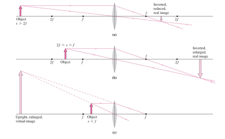
Images with Lenses

1. Converging Lens which bring incoming parallel rays to focus

• Center thickeness is greater than edge thickness

2. Diverging Lens: Bend parallel rays so they appear to diverge from a focus

• Center thickeness is less than edge thickness

• Thin Lens: Thickness is small compared to the curvature of radii of its two surfaces

• Converging Lenses

  • Double convex
  • Planoconvex
  • Convex Meniscus

• Diverging Lenses

  • Double concave
  • Planoconcave
  • Concave Meniscus

• 3 types of principal light rays

  1. parallel to the principal axis
  2. pass through the near focal point
  3. directed at the center of the lens

Converging Lens

• Can produce real and virtual images that are either enlarged or reduced
• 3 distinct cases
  

Diverging Lens

• Virtual image that is upright and reduced in size
  • Virtual image is on the same size as the original object

Thin Lens Equation

$$\frac{1}{s}+\frac{1}{s^{\prime }}=\frac{1}{f}$$

Magnification Equation

$$M=\frac{h^{\prime }}{h}=-\frac{s^{\prime }}{s}$$

Lens Sign Conventions

1. Focal length is positive for converging lenses and negative for diverging lenses
2. The object distance $s$ is positive if it’s on the same side as incoming light rays; negative otherwise
3. The image distance $s^{\prime }$ is positive if the image is on the same side as outgoing light rays
4. The height of the image $h^{\prime }$ is positive if the image is upright and negative if the image is inverted

32: Wave Optics

Light can be viewed in two ways

• As a ray (see the last chapter)
• As a wave (this chapter)

The Wave Nature of Light can be seen through

• Double Slit Experiment
• Single Slit Experiment
• Diffraction

What is Light?

• Light is an electromagnetic wave
  • Shares some similarity to water waves
  • Water also experiences diffraction (spreading out of waves)
  • The reason why light doesn’t experience diffraction in large openings is because light’s wavelength is quite small but most openings are quite large

The wave model

• When light passes through openings smaller than $1$mm, light exhibits wave behavior, so it does spread out
  The Ray Model
• When light passes through openings larger than $1$mm, it behaves like particles and travels in straight lines

Double Slit Experiment

Take a pair of slits, each $0.04$mm wide and spaced around $0.25$ mm apart. The laser beam illuminates both slits. Viewing screen is far behind the slits.

Two separate light waves overlap and interfere, resulting in a pattern of light and dark waves (similar to throwing two stones in water).

A Brief Review of Interference

Constructive Interference: A full-wavelength path difference results in constructive interference.
$$\mathrm{\Delta }r=m\lambda ,m=0,1,2,\dots$$

Destructive Interference: Crest meets trough, means waves cancel. Half-Wavelength path difference leads to destructive interference.
$$\mathrm{\Delta }r=(m+\frac{1}{2})\lambda ,m=0,1,2,\dots$$

Bright Fringes (Constructive Interference)

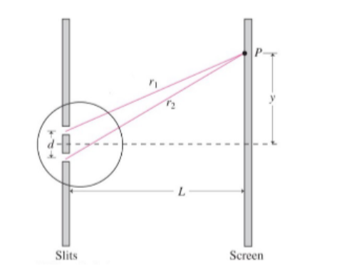
$$\mathrm{\Delta }r=d\sin \theta =m\lambda$$
Note that $\mathrm{\Delta }r$ is the difference between $r_1$ and $r_2$.

To find the actual $y$ position of the fringe, use the following approximation when $\lambda «d«L$
$$\sin \theta =\tan \theta =\frac{y}{L}$$

$$\mathrm{\Delta }r=\frac{dy}{L}=m\lambda$$

$$y_{light}=\frac{m\lambda L}{d}$$

Dark Fringe

$$y_{dark}=\frac{(m+\frac{1}{2})\lambda L}{d}$$

Fringe spacing is
$$\mathrm{\Delta }y=y_m-y_{m-1}=\frac{\lambda L}{d}$$

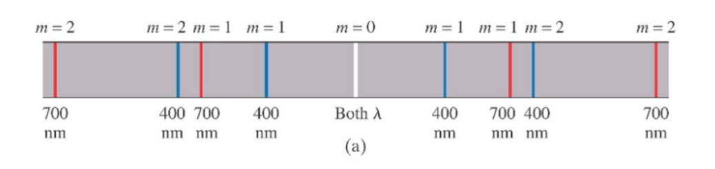
Diffraction Grating

Diffraction Grating (DG): A system with many closely spaced slits

• d: the distance between narrow slits
• N: The number of lines per meter printed on a DG
  $$d=\frac{1}{N}$$

Bright and narrow fringes follows the same rules:
$$d\sin {\theta }_m=m\lambda m=0,1,2,3\dots$$

Consider what happens when white light passes through a diffraction grating.
For all frequencies, the path differences, $\mathrm{\Delta }r=0$ $m=0$. Thus at $m=0$, the light is white. However, at other $m$ values, the path difference for each frequency is different, so each color shows up at different places.

Single Slit Diffraction

• If we send a beam of monochromatic light through a single narrow slit, with viewing screen at distance $L$ and slit width $a$, $L»a$, diffraction occurs
• Unlike with the double slit, there is one large, broad central maximum
• Perfect Destructive Interference- Minima:
  $$a\sin {\theta }_p=p\lambda ,p=1,2,3,\dots$$
• Width of Single-Slit Central Maximum
  $$w=\frac{2\lambda L}{a}$$

Circular-Aperture Diffraction

• Q: What if the rectangular slit is replaced with a hole of diameter $D$?

• A: The diffraction pattern of monochromatic light appears as a central circular max with second bright fringes ringed around

• Angle of first min
  $${\theta }_1=\frac{1.22\lambda }{D}$$

• Width of central maximum
  $$w=2y_1=2L\tan {\theta }_1\approx \frac{2.44\lambda L}{D}$$