Class Information

This course in computational techniques for solving physical problems is for students who have taken PHYS 3511 Scientific Computing II or had extensive previous programming experience. This course covers advanced topics in computational problem solving such as machine learning, probability density function optimization, and Baysian statistical methods, GPU programming. The instructor may add additional topics of interest.

Introduction to Machine Learning

Definitions of ML

• Arthur Sammel (1957): Gives computers the ability to learn without being explicitly programmed
• Tom (1998): A computer program is said to learn from experience, $E$ with respect to task, $T$ with performance, $P$.
  • If performance on $T$ is measured by $P$, it is improved by experience, $E$.

ML Algorithm Types

• Supervised Learning: Give an exact target for each sample during the training process

• Unsupervised Learning: You don’t give the machine an exact target

  • Never give any label during training
  • Machine finds patterns in data on its own

• Reinforcement Learning:

  • It can use supervised and unsupervised algorithms
  • Good for well-defined “playground”
  • Reward good behaviour and punish bad (Learn from mistakes)

• Recommender System: e.g. Youtube recommendations

Supervised Learning

Provide machine with “right answers” train the machine to predict the unknown target

• Regression: Predict continous valued outputs
• Classification: Predict discrete valued outputs

Example 1: Housing Price Prediction

• Cost ($) as a function of Size (Sq ft.)
  • Can be done with regression (linear or nonlinear)
• Cost ($) as a function of Size and Rennovation Cost
  • Multivariable problem with vector representing state value for given input

Example 2: Cancer Diagnosis

• Output (has_cancer): 0 or 1
• Input: Tumor Size
• Problem: Find boundary between “cancer” and “not cancer”
• This is a type of classification problem

Unsupervised Learning

• ML finds patterns in data on its own without explicitly labeling training data with a target

Examples

• Points on a plane, find clusters
• Cluster customers into different groups
• Astronomial data analysis: Find clusters in star/galaxy photo

Regression Problem

• Regression Problem: Predict real-valued output
• Training Set: Data where you know the target value and value for the feature for each point
  • Feature = parameter = input variable
  • Target = output variable you want to predict the value of
• Let $x$ be the features and $y$ be the targets
• Let $m$ be the number of points in the training set
• Let $(x, y)$ denote one training sample and $(x^{(i)}, y^{(j)})$ denote the $i$th training sample
• The learning algorithm generates a hypothesis map/function, $h$, which maps $x$ values to $y$
• Univariate linear regression: Linear regression with one variable (one feature)

Linear Regression

• Choose slope ($\theta_0$) and intercept ($\theta_1$) so that $h(x)$ is close to $y$ and for our training set $(x, y)$

• Hypothesis function
  $$ h_\theta(x^{(i)}) = \theta_0 + \theta_1 x ^{(i)}$$

• Function to minimize
  $$ \frac{1}{2m} \sum_{i=1}^{m} (h_{\theta} (x^{(i)}) - y^{(i)})^2$$

• We use the difference squared since if it wasn’t there could be both positive and negative differences which would lead to a minimized function that isn’t that good

• Cost function
  $$ J(\theta_0, \theta_1) = \frac{1}{2m} \sum_{i=1}^{m} (h_{\theta} (x^{(i)}) - y^{(i)})^2$$

• We want to minimize the cost function

• Consider the case when $\theta_0 = 0$ and when you have 3 points that lie exactly on the line $y = 1 x$

  • For $\theta_1 = 1$, $J(\theta_1) = \frac{1}{2m} \sum_{i=1}^{m} (h_{\theta} (x^{(i)}) - y^{(i)})^2 = \frac{1}{2\cdot 3} (0^2 + 0^2 + 0^2)$
  • For $\theta_1 = 0.5$, $J(\theta_1) \approx 0.58$
  • For $\theta_1 = 0$, $J(\theta_1) \approx 2.3$
  • For $\theta_1 = 1.5$, $J(\theta_1) \approx 0.58$
  • For $\theta_1 = 2$, $J(\theta_1) \approx 2.3$
  • Graphing $J(\theta_1)$ shows that $J(\theta_1)$ is a parabola with only one minimum

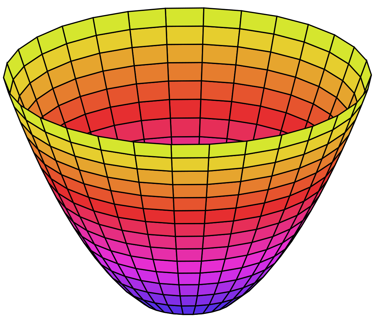
• Considering the multivariable function $J(\theta_1, \theta_0)$ means that the cost function $J(\theta_1, \theta_0)$ is a paraboloid, still with one minimum
  

Gradient Descent

• To find the minimum for $J(\theta_0, \theta_1)$, we can use the Gradient descent algorithm

$$ \text{Repeat until convergence } \left\{ \theta_j := \theta_j - \alpha \pdv{\theta_j} J(\theta_0, \theta_1) \ \ (\text{for j = 0, 1}) \right\} $$

• Make sure to only update $\theta_j$ after everything
• Learning Rate: $\alpha$, controls how big the step size is
  • If $\alpha$ is too large, then there could be divergence
  • If $\alpha$ is too small, then the program might take longer
• If there is a local min as well as a global min for $J(\theta_0, \theta_1)$, one of the problems with the Gradient Descent algorithm is that you might get “stuck” at the local min
  • One solution is to use a larger $\alpha$ value
  • A better solution is to add a “Kinetic Term”. Consider a particle in a well and add kinetic term so particle can oscillate and get out of the well (local minimum)

Gradient Descent for Linear Regression

• Gradient Descent for Linear Regression will always converge since $|\alpha|$ decreases and goes to zero
  $$ \pdv{\theta_j} J(\theta_0, \theta_1) = \pdv{\theta_j} \left[\frac{1}{2m} \sum_{i=1}^m \left(h_\theta (x^{(i)}) - y^{(i)}\right)^2\right] $$
  $$ = \pdv{\theta_j} \left[\frac{1}{2m} \sum_{i=1}^m \left(\theta_0 + \theta_1 x^{(i)} - y^{(i)}\right)^2\right] $$
• For j = 0
  $$ \pdv{\theta_0} J(\theta_0, \theta_1) = \left[\frac{1}{m} \sum_{i=1}^m \left(h_\theta (x^{(i)}) - y^{(i)}\right)\right] $$
• For j = 1
  $$ \pdv{\theta_1} J(\theta_0, \theta_1) = \left[\frac{1}{m} \sum_{i=1}^m \left(\left(h_\theta (x^{(i)}) - y^{(i)}\right)\cdot x^{(i)}\right)\right] $$
• Since we’re not going to use a lot of data, we can use all the samples for each step of GD (“batch processing”)

Linear Regression with Multiple Features

Example: Housing Price

Size	# of Bedrooms	# of Floors	Age of Home	Price ($K)
$x_1$	$x_2$	$x_3$	$x_4$	y
404	5	1	45	460
1416	3	2	40	232
1534	3	2	30	315

• $n=4$ where $n$ is the number of features

• $x^{(i)}$: Input (features) of $i$-th sample

• $x^{(i)}_j$: value of feature j in the $i$-th sample

• Hypothesis:

  • Previous: $h_\theta (x) = \theta_0 + \theta_1 x$
  • Now: $h_\theta (x) = \theta_0 + \theta_1 x_1 + \theta_2 x_2 + \theta_3 x_3 + \theta_4 x_4 + … + \theta_n x_n $

• For convenience of notation, define $x_0 = 1 \implies x^{(i)}_0 = 1$

$$ h_\theta (x) = \underbrace{\theta_0 x_0}_{\text{Bias Term}} + \theta_1 x_1 + \theta_2 x_2 + \theta_3 x_3 + \theta_4 x_4 + … + \theta_n x_n $$

$$ X = \begin{bmatrix} x_0 \\ x_1 \\ x_2 \\ x_3 \\ x_4 \\ \vdots \\ x_n \end{bmatrix} \in \mathbb{R}^{n+1}, \ \ \ \ \Theta = \begin{bmatrix} \theta_0 \\ \theta_1 \\ \theta_2 \\ \theta_3 \\ \theta_4 \\ \vdots \\ \theta_n \end{bmatrix} \in \mathbb{R}^{n+1}$$

$$ h_\theta (x) = \Theta^T X$$

Pseudocode for Multivariable Gradient Descent for Multivariable Linear Regression
$$ \text{Repeat} \left\{ \ \ \ \theta_j := \theta_j - \alpha \frac{1}{m} \sum_{i=1}^m (h_\theta (x^{(i)}) - y^{(i)}) x_j^{(i)}\ \ \ \right\}$$

Eg: $j=0$
$$ \theta_0 := \theta_0 - \alpha \frac{1}{m} \sum_{i=1}^m (h_\theta (x^{(i)}) - y^{(i)}) x_0^{(i)}$$
Eg: $j=2$
$$ \theta_2 := \theta_2 - \alpha \frac{1}{m} \sum_{i=1}^m (h_\theta (x^{(i)}) - y^{(i)}) x_2^{(i)}$$

Feature Scaling

• Examples
  • $x_1$ = size (0 to 2000 sq ft.)
  • $x_2$ = # of bedrooms (1 to 5)
• The problem with the above means there might be problems with gradient descent due to how different the ranges are for each feature
• If you graph $\theta_2$ vs $\theta_1$ without features scaling, you get ellipses around the minimum
• If you graph $\theta_2$ vs $\theta_1$ with features scaling, you get circles around the minimum
• Features have to be on the same scale, roughly $-1 \le x_i \le 1$

Mean Normalization

• Let $\mu_i$ be the mean and $s_i$ be the range

• $x_i’ = \frac{x_i - \mu_i}{s_i}$

• Using the above for the housing price example
  $$x_1 = \frac{\text{size} - 1000}{2000}$$
  $$x_2 = \frac{\text{# of bedrooms} - 3}{5}$$

Logistic Regression - Classification

• Not really used for ML, but an important example of something that gives a non-linear relationship
• Linear Regression doesn’t work for classification problems (Email Spam, Benign Tumor/Cancer)
  • $y \in\{0, 1\}$
  • Gives wrong predictions
  • Linear regression doesn’t confine the values to a specific range

Example: we have data that is either 0 or 1

• We want $0 \le h_\theta(x) \le 1$ (nonlinear function!)
• Define the following
  $$ h_\theta(x) = g (\Theta^T X) = g(z)$$

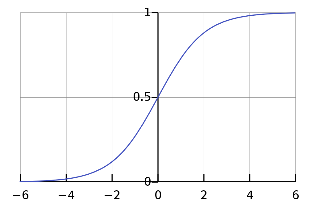
The Sigmoid Function/Logistic Function satisfies this:
$$ g(z) = \frac{1}{1+e^{-z}}$$

Note that
$$ \lim_{z\to\infty} g(z) = 1$$
$$ \lim_{z\to-\infty} g(z) = 0$$
$$ g(0) = \frac{1}{2} $$

Interpretation of $\ h_\theta(x) = g(z)$

• $h_\theta(x)$: Estimated probability that $y=1$ on input $x$

Example

We’re classifying tumors based on size. 1 = Tumor is cancer, 0 = tumor is benign
$$ X = \begin{bmatrix} x_0 \\ x_1 \end{bmatrix} = \begin{bmatrix} 1 \\ \text{Tumor Size} \end{bmatrix}$$
If $ h_\theta(x) = 0.7$, then that means there’s a 70% chance that the tumor is a cancer

Statistical Understanding

Probability that $y=1$, given $x$, parameterized by $\theta$
$$ h_\theta(x) = P(y = 1 | x; \theta)$$

Note the following is true:
$$ P(y = 1 | x; \theta) + P(y = 0 | x; \theta) = 1$$

Decision Boundary

Suppose $h_\theta(x) = g(\Theta^T X)=g(z)$, where $g(z)$ is the sigmoid function

$$ \text{predict } \begin{cases}y = 1 & \text{ if } h_\theta(x) \ge 0.5 \\ y = 0 & \text{ if } h_\theta(x) < 0.5 \end{cases}$$

For the g(z), sigmoid/logistic function:

• $g(z) \ge 0.5$ when $z = \Theta^T X \ge 0$
• $g(z) < 0.5$ when $z = \Theta^T X < 0$

$$ h_\theta(x) = g(\theta_0 x_0 + \theta_1 x_1 + \theta_2 x_2) = g(\theta_0 + \theta_1 x_1 + \theta_2 x_2)$$
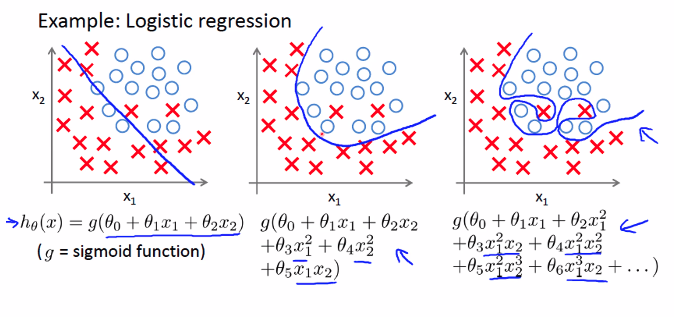
The Line formed by $\theta_0 + \theta_1 x_1 + \theta_2 x_2 = 0$ will form the **decision boundary**

Non-Linear Decision Boundary

The above decision boundary example was linear

• Imagine a data set such that the data is separated into two parts by a decision boundary that is a circle
  $$ h_\theta(x) = g(\overbrace{\theta_0 + \theta_1 x_1 + \theta_2 x_2}^{\text{Linear Terms}} + \underbrace{\theta_3 x_1^2 + \theta_4 x_2^2}_{\text{Non Linear Terms}}) $$

• Example: Radius of circle is 1

  • $x_1^2 + x_2^2 = 1$
    $$ \Theta = \begin{bmatrix} \theta_0 \\ \theta_1 \\ \theta_2 \\ \theta_3 \\ \theta_4 \end{bmatrix} = \begin{bmatrix} -1 \\ 0 \\ 0 \\ 1 \\ 1 \end{bmatrix}$$
    $$ \text{predict } \begin{cases}y = 1 & \text{ if } -1 + x_1^2 + x_2^2 \ge 0 \\ y = 0 & \text{ if } -1 + x_1^2 + x_2^2 < 0 \end{cases}$$

General Decision Boundary With a Lot of Linear Terms

$$ h_\theta(x) = g(\theta_0 + \theta_1 x_1 + \theta_2 x_2 + \theta_3 x_1^2 + \theta_4 x_1^2 x_2 + \theta_5 x_1 x_2^2 + \theta_6 x_1^3 x_2 + …)$$

• The problem with this general problem: What if the decision boundary is simple like a linear line? How do we know beforehand that the decision boundary is linear? We’ll make the decision boundary overly complex with the extra terms if we use the general solution above. Overfitting to be covered in later sections.

Cost Function

$$\text{Training Set } = \{(x^{(1)}, y^{(1)}), (x^{(2)}, y^{(2)}), …, (x^{(m)}, y^{(m)})\}$$
where $m$ is the number of samples

$$ x \in \begin{bmatrix} x_0 \\ x_1 \\ x_2 \\ \vdots \\ x_n \end{bmatrix}$$
$$ h_\theta(x) = \frac{1}{1+e^{-\Theta^T X}}$$

• How do we choose parameter $\theta$?
  $$ J(\theta) = \overbrace{\frac{1}{m}}^{\text{Normalization constant}} \sum_{i=1}^m \text{Cost}(h_\theta (x^{(i)}), y^{(i)})$$
• For linear regression we saw
  $$ \text{Cost}(h_\theta (x^{(i)}), y^{(i)}) = \frac{1}{2} (h_\theta(x^{(i)}) - y^{(i)})^2$$
  $$ \implies J(\theta) = \frac{1}{2m} \sum_{i=1}^m (h_\theta (x^{(i)}) - y^{(i)})^2$$
  • Unlike in linear regression, if we choose $J$ as above with $h_\theta(x)$ as the logistic function, $J$ does not have just one minimum, but might have many local minimums, so $J$ is a **non-convex** function
  • So we have to choose a different cost function and different $J$

Choose $J$ in the following form
$$ J = \sum_{i=1}^m [y^{(i)} J_1 + (1-y^{(i)})J_2]$$
The following does what we want
$$ J = - \frac{1}{M}\sum_{i=1}^m [y^{(i)} \log (h_\theta(x) ) + (1-y^{(i)}) \log(1-h_\theta(x))]$$

• Consider the case when $y=0$ and $h_\theta(x) = 0.99999$ (really bad prediction) as an example of how the above $J$ works well
  • Since the hypothesis function, $h_\theta(x)$ gives a bad prediction, then $J$ approaches $\infty$ as desired

Gradient Descent for Logistic Regression

• Recall that the gradient descent algorithm is the following:
  $$ \text{Repeat until convergence } \left\{ \theta_j := \theta_j - \alpha \pdv{\theta_j} J(\theta_0, \theta_1) \ \ (\text{for j = 0, 1}) \right\} $$
• It turns out the gradient descent algorithm looks exactly the same as for linear regression, just replace $h_\theta(x)$ with the one for logistic regression (See https://math.stackexchange.com/a/477261 for proof)
  $$ \pdv{J(\theta)}{\theta_j} = \frac{1}{m} \sum_{i=1}^m \left(h_\theta(x^{(i)}) - y^{(i)}\right) x_j^{(i)}$$
  $$ \text{Repeat} \left\{ \ \ \ \theta_j := \theta_j - \alpha \frac{1}{m} \sum_{i=1}^m (h_\theta (x^{(i)}) - y^{(i)}) x_j^{(i)}\ \ \ \right\}$$

Conversion to Matrix Form

Note:

• If we have two column vectors, $A$ and $B$, which have dimensions $k \times 1$, then the following is true (see Wikipedia Link):
  $$ A = \begin{bmatrix} a_1 \\ a_2 \\ \vdots \\ a_k \end{bmatrix}, \ \ B = \begin{bmatrix} b_1 \\ b_2 \\ \vdots \\ b_k \end{bmatrix}$$
  $$ A \cdot B = A^T B $$

In the gradient descent algorithm and cost function, $J$, there are a bunch of summations, $\sum$, that must be computed every time we do something

• This is computationally intensive
• Instead, we can convert the summations into matrix multiplication or dot product of column vectors since matrix multiplication/dot products are faste rto compute (especially with libraries like numpy)

Define the following

• $n$: the # of features
• $m$: the # of training samples
• $\mathcal{X}$: The training data represented as a $m \cross n$ matrix
  $$ \mathcal{X} = \begin{bmatrix} x_1^{(1)} & x_2^{(1)} \\ x_1^{(2)} & x_2^{(2)} \\ x_1^{(3)} & x_2^{(3)}\end{bmatrix}$$

In this example, $n=2$ and $m=3$
Note that the matrix of training data, $\mathcal{X}$, is different than the column vector, $X$

Important Matrices and their Dimensions

$$ X = \begin{bmatrix} x_0 \\ x_1 \\ x_2 \\ x_3 \\ x_4 \\ \vdots \\ x_n \end{bmatrix}, \ \ \ \ \Theta = \begin{bmatrix} \theta_0 \\ \theta_1 \\ \theta_2 \\ \theta_3 \\ \theta_4 \\ \vdots \\ \theta_n \end{bmatrix}, \ \ Y = \begin{bmatrix}y^{(1)} \\y^{(2)} \\ \vdots \\ y^{(n)} \end{bmatrix}
, \ \ H_\theta(X) = \begin{bmatrix} h_\theta(x^{(1)}) \\ h_\theta(x^{(2)}) \\ \vdots \\ h_\theta(x^{(n)}) \end{bmatrix} $$

• $\mathcal{X}$: $m \cross n$ (training data set)
• $\Theta$: $n \cross 1$ ($n$ is based on # features)
• $Y$: $m \cross 1$ (Target value for each training sample (row))
• $H_\theta(X)$: $m \cross 1$ vector with $h_\theta(x^{(i)})$ as components. It is the prediction for each $x^{(i)}$ row/sample
• $S$: $n \cross 1$ (# of features), where
  $$ S_j =\sum_{i=1}^{m} (h_\theta(x^{(i)}) - y^{(i)}) x^{(i)}_j $$

Then we have the following equivalencies:

$$ \Theta^T X = \Theta \cdot X $$
$$ S_j = \sum_{i=1}^{m} (h_\theta(x^{(i)}) - y^{(i)}) x^{(i)}_j \implies S = \mathcal{X}^T H = \mathcal{X} \cdot H$$

Gradient Descent Algorithm in Matrix Form

We can then rewrite the gradient descent algorithm as follows:
$$ \text{Repeat} \left\{ \ \ \ \theta_j := \theta_j - \alpha \frac{1}{m} \sum_{i=1}^m (h_\theta (x^{(i)}) - y^{(i)}) x_j^{(i)}\ \ \ \right\} $$
$$ \implies \text{Repeat} \left\{ \ \ \ \theta_j := \theta_j - \alpha S_j \ \ \ \right\}$$
$$ \implies \text{Repeat} \left\{ \ \ \ \Theta := \Theta - \alpha S \ \ \ \right\}$$

Other Optimization Algorithms

Conjugate Gradient

• Popular a lot for Computational Chemistry/Material Science (DFT)
• Google “BFGS” and “L-BFGS”

Advantages

• No need to manually pick $\alpha$
• Often faster than gradient descent (GD)

Disadvantages

• More complex
• A lot of other parameters
  • Parameter akin to Speed of particle on potential
  • Paremeter akin to Random motion of particle

Multi Classification Problem

• Instead of just a binary classification (yes, no), what if we want to classify data into more than just two categories

Example

• Email Tagging: Classify inbox into Work emails ($y=1$), friend emails ($y=2$), family email ($y=3$), hobby emails ($y=4$)

One vs. All (One vs. Rest)

• You can reuse the binary classification algorithm to classify data into $y=1$ and $y\neq 1$
• Then afterwards, classify the $y\neq 1$ data into $y=2$ and $y\neq2$
• Repeat

OverFitting

• Options to address overfitting

1. Reduce number of features
   • Manually select which features to keep (requires domain knowledge to know which ones to keep and which ones are less important)
   • Model Selection Algorithm
2. Regularization
   • Want to make $\theta_j$ for higher order terms small
     $$ J_\theta - [ \frac{1}{m} \sum_{i=1}^m y^{(i)} ]$$

Gradient Descent for Logistic Regression

Repeat {
$$ \theta_0 := \theta_0 - \alpha \frac{1}{m} \sum_{i=1}^m (h_\theta (x^{(i)}) - y^{(i)}) x_0^{(i)}$$
$$ \theta_j := \theta_j - \alpha \frac{1}{m} \sum_{i=1}^m (h_\theta (x^{(i)}) - y^{(i)}) x_j^{(i)} + \frac{\lambda}{m} \theta_j, \ \ j = 1, 2, 3, 4, \cdots n$$
}

K-Means Cluster - Unsupervised Learning

Uses

• Film Recommendation

• Social Network, Finding similarities between users

  • Represent each user as node in graph, with connection as edge

• Materials Science, represent each material as node with properties as edges

• Cluster

Algorithm

• Input
  • Number of Clusters (K)
  • Training Set: $\{x^{(1)}, x^{(2)}, …, x^{(m)}\}$
    • $m$ is number of samples

1. Randomly pick $K$ cluster centroids, $\mu_1, \mu_2, …, \mu_k \in \mathbb{R}^k$

   • Sometimes more efficient to choose $K$ samples as the centroids

2. Repeat {
   // Cluster Assignment
   for i=1 to m:
   $c^{(i)}$:= index of cluster centroid closest to $x^{(i)}$

   // Move Centroid
   for k=1 to K:
   $\mu_k$:= average (mean) of all the points assigned to cluster $k$
   }

Example:

• $x^{(1)}, x^{(5)}, x^{(6)}$
• Suppose $c^{(1)} = 3, \ c^{(5)} = 3, \ c^{(6)} = 3$
• Then $\mu_3 = \frac{1}{3} (x^{(1)}+ x^{(5)}+ x^{(6)})$

Optimization Objective

$$J(c^{(1)}, …, c^{(m)}, \mu_1, …, \mu_k) = \frac{1}{m}\sum_{i=1}^m |x^{(i)} - \mu_{c^{(i)}}|^2$$

• Want to minimize $J$
  1. Minimize J with respect to $c^{(1)}, …, c^{(m)}$ while holding $\mu_1, …, \mu_k$ constant
  2. Minimize J with respect to $\mu_1, …, \mu_k$ while holding constant $c^{(1)}, …, c^{(m)}$

Random Initialization

1. Randomly pick $K$ samples $K < m$
2. Set $\mu_1, \cdots \mu_k$ equal to the above $K$ samples

What is the right value of K

• Graph of J vs. K should give you an obvious “elbow” point (drops steeply) and then drops smoothly and less steeply afterwards

  • The $K$ value for the elbow point should be the one to choose (most of the time)

  • However, sometimes the graph doesn’t drop steeply. This means you have too many features or that the K-means algorithm itself is not a good algorithm to use in this case

PCA (Principle Component Analysis)

• If we have too many features (too many dimensions) when doing K-means algorithm, we can reduce to fewer dimensions
• PCA, Kernel PCA, ICA: “Powerful unsupervised learning techniques for extracting hidden (potentially lower dimensional) structure from high dimensional datasets”
• In the data cleaning step of workflow

Uses

• Visualization
• More efficient (time, memory, etc.)
• Fewer dimensions implies better generalizations
• Noise Removal

Idea

• Want to pick the most important features (principle components)
• Project the data onto the principle component axis(es) so that variance among data is maximized
• Alternatively: Find a direction (a vector $u^{(1)} \in \mathbb{R}^n$) onto which to project the data so as to minimize the projection error/distance

A Tutorial on Principal Component Analysis by Jonathon Shlens

Algorithm

• Reduce from $n$-dimensions to $k$-dimensions
• Find $k$ vectors $u^{(1)}, u^{(2)}, u^{(3)}, …, u^{(n)}$ onto which to project the data
• Compute"Covariance Matrix”, $\Sigma$
  $$ \Sigma = \frac{1}{m}\sum_{i=1}^n (x^{(i)}) (x^{(i)})^T$$
• $\Sigma$ yields an $n\cross n$ matrix
• Calculate eigenvectors of the covariance matrix, $\Sigma$
  $$[U, S, V]= \text{Singular Value Decomposition}$$
  • where the columns of $U$ make up the principle components
    • First column of U, $u^{(1)}$ is PC1 (Principal Component 1)
    • Second column of U, $u^{(2)}$ is PC2
    • And so on until $u^{(n)}$

Example: Supervised Learning Speedup

*$m$ Samples: $(x^{(1)}, y^{(1)}), (x^{(2)}, y^{(2)}), (x^{(3)}, y^{(3)}),…, (x^{(m)}, y^{(m)})$

• Suppose there are 1000 features

• Extract inputs and unlabaled dataset: $x^{(1)}, x^{(2)}, … ,x^{(m)} \in \mathbb{1000}$

• Do PCA to reduce dimensions from training set $x$ to $z$
  $$z^{(1)}, z^{(2)}, … ,z^{(m)} \in \mathbb{1000}$$

• New training Set has features reduced: $(z^{(1)}, y^{(1)}), (z^{(2)}, y^{(2)}), (z^{(3)}, y^{(3)}),…, (z^{(m)}, y^{(m)})$

Difference/Connection Between SVD and PCA

• PCA transforms data linearly into a new set that are not correlated (orthgonal)
• SVD is a method in linear algebra used to diagonalize a matrix into special matrices
• We use SVD to find PCs (Principle Axises in PCA)

Matrix Diagonalization

• For some square matrices, $A$: $n \cross n$
  $$ A = V \lambda V^{-1}$$

• where each column in $V$ gives you the eigenvectors

• And $\lambda$ is a diagonal matrix with the eigenvalues corresponding to the eigenvectors

• $V$ and $V^{-1}$ are orthogonal

Singular Value Decomposition

For any matrix, $A$ is $m \cross n$

• $m$ is the number of samples

• $n$ is the number of features

• $AA^{T}$ is the covariance matrix ($m \cross m$)

• $ A^T A$ ($n \cross n$)

• $AA^T \to u_i$ as eigenvectors

• $A^T A \to v_i$ as eigenvectors $\to $ singular vectors

• $U$ is the covariance matrix with $u_i$ as columns

• $V$ is the matrix with $v_i$ as columns

• SVD states that any matrix $A$ can be written as follows
  $$ A = US V^T$$

  • $S$ is a diagonal matrix with singular values $\sigma_i = \sqrt{\underbrace{\lambda_i}}_{\text{eigenvalue from }U}$

  $$ A_{m \cross n} = U_{m\cross m} S_{m\cross n} V^T_{n \cross n}$$

• Each $u_i$ in the $U$ matrix corresponds to the principle components

  • we can order the eigenvectors so that the higher eigenvalues come first
  • Higher eigenvalues mean larger variance (so more important PC)
  • You can then project the data onto the first few PCs since the $u_i$ give the axises

Neural Networks: Non Linear Classification Example

• Using a neural network is a solution for non linear regression or classification problems with a large number of features

• Using the sigmoid function is not feasible since the number of nonlinear terms in $z$ for $g(Z)$ is too much

Neuron Model

• Each neuron can have multiple inputs (can be from other neurons). Depending on the current strength, the neuron fires
  • Non linear activation!
• Inputs: $x_1, x_2, x_3$
  • The wires coming into the neuron are how heavily weighted each input is, in other words, $\theta_1, \theta_2, \theta_3, \cdots$ corresponding with each $x_1, x_2, x_3, \cdots$
  • The output is $h_\theta(x) = \frac{1}{1+e^{-\Theta^T X}}$ based on the input, $x_i$ and input weights ($\theta_i$)
    • The sigmoid function is the activation function

$$ X = \begin{bmatrix} x_0=1 \\ x_1 \\ x_2 \\ x_3 \end{bmatrix}, \ \ \ \theta^{(j)} = \begin{bmatrix} \theta_0^{(j)} \\ \theta_1^{(j)} \\ \theta_2^{(j)} \\ \theta_3^{(j)} \end{bmatrix}$$

Example

• $a_i^{(j)}$ = “activation” of unit $i$ in layer $j$
• $a^{(2)}_3$ means the 3rd node in the 2nd layer
• $\theta^{(j)}$ = vector of weights controlling function mapping from layer $j$ to $j+1$
  $$ a_1^{(2)} = g(\theta_{10}^{(1)} x_0 + \theta_{11}^{(1)}x_1 + \theta_{12}^{(1)} x_2 + \theta_{13}^{(1)} x_3) = g(z_1^{(2)}) $$
  $$ a_2^{(2)} = g(\theta_{20}^{(1)} x_0 + \theta_{21}^{(1)}x_1 + \theta_{22}^{(1)} x_2 + \theta_{23}^{(1)} x_3) = g(z_2^{(2)}) $$
  $$ a_3^{(2)} = g(\theta_{30}^{(1)} x_0 + \theta_{31}^{(1)}x_1 + \theta_{32}^{(1)} x_2 + \theta_{33}^{(1)} x_3) = g(z_3^{(2)}) $$
• $\theta_j$ is a vector with dimension $ 1 \times (s_{j+1} \cdot (s_j + 1))$ , where $j$ layer and $s_j$ is the number of nodes at layer $j$
  • $\theta^{(1)} = 3 \times (3+1) = 12$
  • $\theta^{(2)} = 1 \times (3+1) = 4$

Forward Propogation: Vectorized Implementation

$$ X = \begin{bmatrix} x_0=1 \\ x_1 \\ x_2 \\ x_3 \end{bmatrix}, \ \ z^{(2)} = \begin{bmatrix} z_1^{(2)} \\z_2^{(2)} \\z_3^{(2)} \end{bmatrix}$$
$$z^{(2)} = \theta^{(1)} X$$
$$ a^{(2)} = g(z^{(2)})$$
$$a_0^{(2)} = 1 \implies z^{(3)} = \theta^{(2)} a^{(2)}$$
$$ \implies z^{(3)} = \theta^{(2)} a^{(2)}$$
$$ \implies h_\theta(x) = a^{(3)} = g(z^{(3)})$$

The general steps for forward propogation:
$$ x \longleftrightarrow a^{(1)} \xrightarrow[\theta^{(1)}]{} z^{(2)} \xrightarrow[g(z^{(2)})]{} a^{(2)} \xrightarrow[\theta^{(2)}]{} z^{(3)}\xrightarrow[g(z^{(3)})]{} a^{(3)} \longleftrightarrow h_\theta(x) $$

• You can cut unimportant features with small weights. Called “dropout”

• $\theta^{(1)}$: New Feature Generation

• If instead of each $a^{(j)}_i$, we used $z^{(j)}_i$, we would basically just do linear regression since the output node would just be linear terms

Example: And Gate

Activation Functions

• Sigmoid Function (from 0 to 1)
• Hyperbolic Sin (from -1 to 1)
• Rectified Linear (relu)
• Softmax
  • Can be viewed as a screening function
  • Picks out the most important/dominant components of a vector and assign larger values to those components

Bayesian Statistics and Naive Bayes Learning

• Sometimes we don’t have the “big data” needed for the algorithms used above
• If you don’t have a lot of data, you can use Bayesian Statistics and Naive Bayes Learning
  • But if you do have a lot of data, use the above big data techniques
• Example: Recommender System
• $P(y|x)$ Disriminative
  • $P(y|x)$ is “probability of y given x”
• $P(y|x)$ Generative
  • $P(y|x)$ is “probability of x given y”
  • $y$ in our example is either $0$ or $1$
  • $x$ in our example is the feature in the 2d space ($x_1$ or $x_2$)
  • $P(x|y=1)$ and $P(x|y=0)$
  • Asks the Question: What are the features like if $y= \{0, 1\}$?

Conditional Probability

• $ P(A|B)$: Given that $B$ has occured, what is the probability that event $A$ occurs?
  $$ P(A|B) = \frac{P(A \cap B)}{P(B)}$$

Example

The % of adults who are male and alcoholics is 2.25%. What is the probability of being alcohol, given being a man?

$$ A = \text{being an alcoholic}$$
$$ B = \text{person is a male}$$
$$ P(A \cap B) = 2.25\% $$
$$ P(A | B) = \text{prob of person being an alcoholic given they are male}$$
$$ P(A|B) = \frac{P(A \cap B)}{P(B)} = \frac{0.0225}{0.5} = 0.045 = 4.51 \%$$

Bayes’ Theorem

$$ P(A|B) = \frac{P(A \cap B)}{P(B)}$$
$$ P(B|A) =\frac{P(B \cap A)}{P(A)} $$
$$ \implies P(A|B) \cdot P(B) = P(B | A) \cdot P(A) $$
$$ \implies P(A|B) = \frac{P(B|A) \cdot P(A) }{P(B)}$$

Example

What is the probability of a family with two girls given that the family has at least one girl?

• GG, GB, BG, BB
  • 3/4 of the above cases have at least one girl
  • 1/4 of the cases above have two girls
  • P=1/3 for probability that a family has two girls given at least one girl
• Now using Bayes’ Theorem
  $$ P(2G | 1G) = \frac{P(1G|2G) \cdot P(2G)}{P(1G)} = \frac{1 \cdot \frac{1}{4}}{\frac{3}{4}} = \frac{1}{3}$$

Using Bayesian Statistics for Recommender Systems

• Suppose we know $P(x|y)$ and $P(y)$
• Given new $x$
  $$P(y=1|x)$ = \frac{P(x|y=1) \cdot P(y=1)}{P(x)}$$
  $$ P(x) = \sum_y P(x, y) = P(x|y=1) \cdot P(y=1) + P(x|y=0) \cdot P(y=0)$$
  $$ P(y=1) + P(y=0) = 1$$

Example

$$ P(x|y=0) = 0.01$$
$$ P(x|y=1) = 0.03$$
$$ P(y=1) = P(y=0) = 0.5$$
Question: What is the probability that for a new sample $P(y=1| x)$

$$ P(y=1 | x) = \frac{P(x|y=1)\cdot P(y=1)}{P(x|y=1) \cdot P(y=1) + P(x|y=0) \cdot P(y=0)}$$
$$= \frac{0.03\cdot 0.5}{0.03\cdot 0.5 + 0.01\cdot 0.5} = 0.75$$

Naive Bayes Example: Text Classification

• Given: Feature vector $x$, $P(x|y)$, $P(y|x)$
  $$ x = \begin{bmatrix}0 \\ 0 \\ 0 \\ \vdots \\ 1 \\ \vdots \\ 0 \\ 0 \\ 0 \\ 0 \end{bmatrix} $$
• The feature vector describes the number of occurences of a word or probability of the word appearing (sort of like a hashmap)
• For this example:
  $$x_i = \begin{cases} 1 & \text{if word }i \text{ of dictionary appears in the text}\\ 0 \end{cases}$$

$$ P(x|y) =\prod_{i=1}^n P(x_i| y) $$

• Then compare $P(x|y=1)$ vs. $P(x|y=0)$ to get recommendation
  • e.g. $0.000005 > 0.000003$

Atomic Simulations

Why Simulate?

• “Computers don’t solve problems, people do” (Frank Jensen)
• Simulations rarely simulate reality
  • Simulations mainly compute quanitites that will either prove or disprove a theory

Energy Models

• Empirical Models (parameters fitted to experimental data)
  • Fastest
  • Many body potentials
  • Pair potentials
• Semi-Empirical
  • Tight Binding
• Quantum Mechanical (start from Schrodinger’s equation and make approximations)
  • Slowest
  • Quantum chemistry
    • Based on atomic orbitals
  • Density Functional Theory (DFT)
  • Quantum Monte Carlo

Born Oppenheimer Approxmation

• All atoms characterized by coordinate vector $\vec{R}_i$
• System characterized by wavefunction $\psi$

Born Oppenheimer Approximation

• The wavefunctions of the nuclei and electrons can be treated separately since the nuceli are a lot heavier than the electrons

Pairwise Energy Summation: Pair Potential

$$ E = (E_0) + \frac{1}{2} \sum_{i, j \neq i}^N V(\vec{R}_i - \vec{R}_j)$$

Formation Energy of Crystals

• Amount of energy that holds a crystal together
• Formation energy is always negative

Density Functional Theory

• All system properties can be represented as a function of electron density, which in turn can be represented by wavefunctions

Band Gap